| Issue |
A&A
Volume 580, August 2015
|
|
|---|---|---|
| Article Number | A124 | |
| Number of page(s) | 23 | |
| Section | Astrophysical processes | |
| DOI | https://doi.org/10.1051/0004-6361/201526104 | |
| Published online | 17 August 2015 | |
Temperature-averaged and total free-free Gaunt factors for κ and Maxwellian distributions of electrons⋆
1
Department of Mathematics University of Évora,
R. Romão Ramalho 59,
7000
Évora,
Portugal
e-mail:
This email address is being protected from spambots. You need JavaScript enabled to view it.
2
Zentrum für Astronomie und Astrophysik, Technische Universität
Berlin, Hardenbergstrasse
36, 10623
Berlin,
Germany
e-mail:
This email address is being protected from spambots. You need JavaScript enabled to view it.
Received: 16 March 2015
Accepted: 6 May 2015
Abstract
Aims. Optically thin plasmas may deviate from thermal equilibrium and thus, electrons (and ions) are no longer described by the Maxwellian distribution. Instead they can be described by κ-distributions. The free-free spectrum and radiative losses depend on the temperature-averaged (over the electrons distribution) and total Gaunt factors, respectively. Thus, there is a need to calculate and make available these factors to be used by any software that deals with plasma emission.
Methods. We recalculated the free-free Gaunt factor for a wide range of energies and frequencies using hypergeometric functions of complex arguments and the Clenshaw recurrence formula technique combined with approximations whenever the difference between the initial and final electron energies is smaller than 10-10 in units of z2Ry. We used double and quadruple precisions. The temperature-averaged and total Gaunt factors calculations make use of the Gauss-Laguerre integration with 128 nodes.
Results. The temperature-averaged and total Gaunt factors depend on the κ parameter, which shows increasing deviations (with respect to the results obtained with the use of the Maxwellian distribution) with decreasing κ. Tables of these Gaunt factors are provided.
Key words: atomic processes / radiation mechanisms: general / ISM: general / galaxies: ISM
Appendices are available in electronic form at http://www.aanda.org
© ESO, 2015
1. Introduction
Astrophysical plasma emission codes are a powerful tool for calculating spectra and energy losses in a plasma such as the interstellar or intergalactic medium and for comparing the results with observations. However, such plasmas are complex systems in which frequently made assumptions, like establishing the Maxwell-Boltzmann distribution (hereafter referred as Maxwellian distribution) of the electrons and ions, are not always fulfilled and may lead to erroneous interpretations of the plasma properties. We have therefore reexamined the nonrelativistic free-free Gaunt factor, which is the quantum correction for the semiclassical cross section of Kramers (1923). The factor has been the subject of many papers over the years, comprising analytical approximations (e.g., Menzel & Pekeris 1935; Elwert 1954; Grant 1958; Brussaard & van de Hulst 1962; Hummer 1988; Beckert et al. 2000) to the exact quantum mechanical expressions (in terms of hypergeometric functions) derived, for example, by Menzel & Pekeris (1935), Sommerfeld (1953, using nonrelativistic dipole approximation), Kulsrud (1954), and Biedenharn (1956), and detailed numerical computations first discussed in the seminal work of Karzas & Latter (1961, hereafter KL61) and followed by a series of publications during the past five decades.
Karzas & Latter computed the Gaunt factor using hypergeometric functions of complex variables and presented their results in graphical form. The problem reduces to calculating the solution of differential equations by means of power series of the real variable x (which is negative) at two regimes (|x| > 1 and |x| ≤ 1) with a very slow convergence when |x| → 1. Since KL61, several authors recalculated the Gaunt factor with increasing precision and size of parameter space (e.g., O’Brien 1971; Carson 1988; Hummer 1988; Nicholson 1989; Janicki 1990; Sutherland 1998; van Hoof et al. 2014). Special care was taken to overcome the slow convergence of the solution by (i) redefining the regimes through a change in variables (O’Brien 1971), which has been adopted, in combination with KL61 formulae, in most of the calculations that followed; (ii) increase in precision; and (iii) by using the approximation of Menzel & Pekeris (1935, see discussion in van Hoof et al. 2014.
The Gaunt factor can be averaged over a distribution of electrons (also known as the temperature-averaged Gaunt factor) and then integrated over the full range in frequency (the total Gaunt factor). These in turn are used in the determination of the emission spectra and radiative losses by a plasma as a result of this process. In general, the averaging is made over a Maxwellian distribution of electrons, thus relying on the assumption that thermal equilibrium is the rule (see, e.g., Karzas & Latter 1961; Gayet 1970; Armstrong 1971; Feng et al. 1983; Carson 1988; Hummer 1988; Nicholson 1989; Janicki 1990; Sutherland 1998; van Hoof et al. 2014).
However, this condition may not be attained if high-energy electrons are injected into the system on timescales shorter than that needed to achieve thermalization (Livadiotis & McComas 2009) or when long-range forces are present in the plasma (Collier 2004). Deviations may also occur in the presence of strong temperature and/or density gradients (Collier 1993; Collier et al. 2004, see discussion in, e.g., Dudík et al. 2011 and references therein). An example of nonthermal distributions is the so-called κ-distribution, which was first used by Vasyliunas (1968) to match the observed electron distribution in the Earth’s magnetosphere. κ-distributions have also been used to explain the discrepancies observed in the abundances and temperatures in Hii regions and planetary nebulae when derived using collisional excitation lines and optical recombination lines (see Binette et al. 2012; Nicholls et al. 2012, 2013). The κ-distribution is characterized by a high-energy power-law tail and has the form ![Mathematical equation: \begin{equation} f_{\kappa}(E){\rm d}E=\frac{2E^{1/2}}{\pi^{1/2}(k_{\rm B}T)^{3/2}} \displaystyle A_{\kappa} \left[ 1+\frac{E}{(\kappa-3/2)k_{\rm B}T}\right]^{-\kappa-1}{\rm d}E, \end{equation}](/articles/aa/full_html/2015/08/aa26104-15/aa26104-15-eq8.png) (1)with
(1)with  (2)and Γ(x) denoting the gamma function of the variable x. When κ → ∞, the Maxwellian distribution is recovered. As κ decreases, deviations from the Maxwellian distribution increase, reaching maximum when κ approaches 3/2 (Fig. 1, which displays the κ and Maxwellian distributions at different temperatures for electrons with energies varying between 10-2 and 104 eV). Similarly to the Maxwellian distribution, the mean energy of the κ-distribution is independent of κ and is given by ⟨ E ⟩ = 3 / 2kBT. Hence, T can be defined as the thermodynamic temperature for these distributions. For a review of the κ-distribution and its applications see Pierrard & Lazar (2010) and Livadiotis & McComas (2009).
Dudík et al. (2011, 2012) calculated the free-free contribution to the emission spectra and to the radiative losses of a plasma with the nonthermal distributions (κ and n distributions) and evolving under collisional ionization equilibrium conditions (CIE), that is, the number of recombinations equals the number of ionizations by electron impact. The authors calculated the temperature-averaged Gaunt factors for nonthermal distributions using the free-free Gaunt factors of Sutherland (1998).
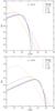 |
Fig. 1 Not normalized Maxwellian and κ-distributions (with different κ) at 104 K (top) and 106 K (bottom panel). The largest deviation of the Maxwellian distribution occurs for the lowest κ, showing an increase in electrons at the low- and high-energy ranges when compared to the Maxwellian distribution. |
The temperature-averaged and total Gaunt factors are needed for detailed simulations involving the coupling of the dynamical and thermal evolutions of the interstellar medium, bubbles and superbubbles (including the Local Bubble), and formation of galaxies, to name just a few. Hence, we carried out detailed calculations of the free-free Gaunt factor and of the temperature-averaged and total Gaunt factors for Maxwellian and κ-distributions (considering a large grid of κ parameters). We present these results in tabulated form to be used in any plasma emission software through convenient one- and two-dimensional interpolations.
The structure of this paper is as follows: Sect. 2 describes the calculation of the free-free Gaunt factors. Section 3 deals with the temperature-averaged and total Gaunt factor for Maxwellian and κ distributions of electrons. Section 4 describes the tabulated data, and we conclude in Sect. 5 with some final remarks.
2. Calculations of the Gaunt factor
The calculation of the free-free Gaunt factor in double and quadruple precision follows the prescription of Janicki (1990) with some adaptations taken from Carson (1988) and van Hoof et al. (2014). It is assumed that an electron with initial energy Ei absorbs a photon of energy hν. Thus, the electron transits to a higher state with an energy Ef = Ei + hν. The free-free Gaunt factor is then given by (KL61) ![Mathematical equation: \begin{equation} g_{_{\rm ff}}= \frac{2\sqrt{3}}{\pi}I_{0}\left[I_{0}\left(\frac{\eta_{\rm i}}{\eta_{\rm f}}+\frac{\eta_{\rm f}}{\eta_{\rm i}}+2\eta_{\rm i}\eta_{\rm f}\right)-2I_{1}\sqrt{1+\eta_{\rm i}^{2}}\sqrt{1+\eta_{\rm f}^{2}}\right], \end{equation}](/articles/aa/full_html/2015/08/aa26104-15/aa26104-15-eq23.png) (3)where
(3)where  , ϵi = Ei/Z2Ry and ϵf = Ef/Z2Ry are the electron scaled initial and final energies, respectively; Ry is the infinite-mass Rydberg unit of energy, and Z the atomic number of the ion. The functional Il (with l = 0.1) is defined as
  (4)where Gl is a real function given by
  (5)with x = −4ηiηf/ (ηi − ηf)2 (which is always negative), a = l + 1 − iηf, b = l + 1 − iηi, and c = 2l + 2;
  is the hypergeometric function, which satisfies the equation
 ![Mathematical equation: \begin{equation} x(1-x)F^{\prime\prime}+\left[c-(a+b+1)x\right]F^{\prime}-abF=0. \end{equation}](/articles/aa/full_html/2015/08/aa26104-15/aa26104-15-eq39.png) (6)Gl satisfies the equation (Janicki 1990)
(6)Gl satisfies the equation (Janicki 1990)  (7)with f1 = c + x(2d − a − b − 1) and f2 = x [ d2 + ab − d(a + b) ] − ab + dc. Thus, the free-free Gaunt factor determination reduces to the calculation of solutions for Gl, and therefore for Il, for l = 0, 1 in terms of a power series in x for |x| < 1 and in y = −1 /x for |x| > 1 (KL61). These solutions converge very slowly near 1, but a change in variables to (Janicki 1990)
  (8)facilitates the calculation. The threshold results from equating |x| / (|x| − 1) to −1 / |x| and taking into account that x< 0 (see text above). Another step comprises the usage of the Clenshaw recurrence formula to calculate Gl at each regime by means of a series of terms. The number of terms n to be considered in the sum to within a certain precision, for example, 10− δ, is given by −δ/ log |x/ (x − 1)| (for |x| ≤ 1.61804) and −δ/ log | − 1 /x| (|x| > 1.61804). For further details see Janicki (1990).
In the range  , with w = ϵf − ϵi = hν/Z2Ry, the exact solution fails (see Carson 1988; Hummer 1988; van Hoof et al. 2014). Hence, the approximation of Menzel & Pekeris (1935) with the correction by van Hoof et al. (2014) is used:
 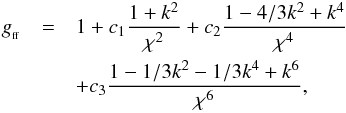 (9)with k = ηf/ηi, χ = [(1 − k2)ηf]1 / 3, c1 = 0.1728260369..., c2 = −0.04959570168..., and c3 = −0.01714285714.... The maximum error in this approximation is smaller than 5.5 × 10⁻¹⁰ (van Hoof et al. 2014).
Figure 2 displays the variation of the free-free Gaunt factor with the normalized initial electron energy (top panel) for specific photon energies running from log (hν/z2Ry) = 8 through −4 with steps of dex = 1, and with the normalized photon energy (bottom panel) for initial electron energies of log (Ei/z2Ry) = −5 through 8 with steps of dex = 1. These Gaunt factors overlap with those reported by van Hoof et al. (2014) and Sutherland (1998).
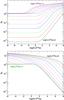 |
Fig. 2 Free-free Gaunt factor variation with the normalized initial electron energy (top panel) for specific photon energies running from log hν/z2Ry = 8 through −4 with steps of dex = 1, and with the normalized photon energy (bottom panel) for initial electron energies of log Ei/z2Ry = −5 through 8 with steps of dex = 1. |
3. Temperature-averaged and total Gaunt factor
The energy spectrum by free-free emission from electrons with an energy distribution f(E) is given by (see, e.g., Kwok 2007) 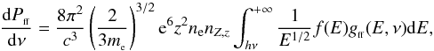 (10)where ν is the frequency of the emitted photon, T is the temperature, kB is the Boltzmann constant, ne is the electron density,
  is the number density of ion with atomic number Z and ionization stage z. For electrons with a κ or Maxwellian (κ → ∞) distribution, and after a suitable change of variables, Eq. (10) becomes
 ![Mathematical equation: \begin{eqnarray} \label{power} \frac{{\rm d}P_{_{\rm ff}}}{{\rm d}u} &=& C_{_{\rm ff}} z^{2} n_{\rm e} n_{_{Z,z}} T^{1/2} \times \\ & \times & \left\{ \begin{array}{lllc} \displaystyle \int_{0}^{+\infty}g_{_{\rm ff}}(\gamma^{2},u)\frac{A_{\kappa}}{\left[1+\frac{x+u}{\kappa-3/2}\right]^{\kappa+1}}{\rm d}x & {\rm if} & \kappa> 3/2 \\ && \nonumber\\ \displaystyle {\rm e}^{-u} \int_{0}^{+\infty}g_{_{\rm ff}}(\gamma^{2},u){\rm e}^{-x}{\rm d}x & {\rm if} & \kappa\to \infty, \end{array}\right. \end{eqnarray}](/articles/aa/full_html/2015/08/aa26104-15/aa26104-15-eq78.png) (11)where
(11)where  , and the parameters x, u and γ have the forms
  (12)The integral on the right-hand side of Eq. (11) is the temperature-averaged Gaunt factor (KL61). Integration of Eq. (11) over the photon frequency spectrum gives the total free-free power associated with an ion (Z,z)
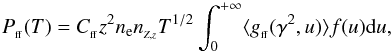 (13)with f(u) = e− u (for κ → ∞; Maxwellian distribution) and f(u) = 1 for κ> 3 / 2 (κ distribution). The total free-free Gaunt factor is defined as (see, e.g., KL61)
 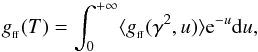 (14)and, thus, can be calculated for both distributions.
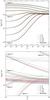 |
Fig. 3 Temperature-averaged Gaunt factors calculated for κ = 2, 5, 10, 15, and 25) and Maxwellian distributions of electrons for the range 10-4 ≤ γ2 ≤ 104 (top panel) and zoomed-in to the region γ2 ∈ [ 102,104 ] and ⟨ gff(γ2,u) ⟩ ∈ [ 0.8,2 ] (bottom panel). |
Figures 3 and 4 display the variation with γ2 of the temperature-averaged, ⟨ gff(γ2,u) ⟩, and total free-free, gff(T) Gaunt factor. The results correspond to κ = 2, 5, 10, 15, 25 and ∞ (the latter value corresponds to the Maxwellian distribution).
The temperature-averaged Gaunt factors depend on the κ parameter - with the decrease of κ, the deviations of ⟨ gff(γ2,u) ⟩ increase with respect to the Maxwellian-averaged value (Fig. 3). The strongest deviation always occurs for κ → 3 / 2. These deviations depend strongly on the γ2 (i.e., on the temperature) and mildly on the u (i.e., on the frequency) parameters. As γ2 tends to −∞, the ⟨ gff(γ2,u) ⟩ for different κ approximates the Maxwellian-averaged value (black dashed line; top panel of Fig. 3), which also depends on the value of u. With the decrease of u (for u< 1) the degree of blending among the temperature-averaged Gaunt factors diminishes. With an increase in γ2 (decrease in temperature), the deviations become larger and more pronounced for γ2> 10 (bottom panel of Fig. 3). However, regardless of the value of γ2 , the ⟨ gff(γ2,u) ⟩ shows a small variation for all κ ≥ 5 even for γ2> 10.
The total Gaunt factor shows a similar dependence on κ for the different γ2 as ⟨ gff(γ2,u) ⟩. That is, the deviations increase with increasing γ2 (Fig. 4). The total Gaunt factor maximum decreases with increasing κ from 2.038 to 1.441 for κ = 2 and κ → ∞, respectively. When γ2 → ∞, the total Gaunt factor tends to 1.596 for κ = 2, decreasing toward 1.0 with κ → ∞ (the Maxwellian distribution). With γ2 → −∞gff(T) → 1.224 and 1.1 for κ = 2 and κ → ∞, respectively.
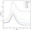 |
Fig. 4 Total free-free Gaunt factor calculated for κ (2, 3, 5, 10, 15, and 25) and Maxwellian distributions. The maximum of gff(T) moves to the left with the increase in κ. |
As the total Gaunt factor decreases with increase in κ, the losses of energy due to free-free emission follow the same path as a result of Eq. (13).
4. Tables
Temperature-averaged and total free-free Gaunt factors calculated for κ (2, 3, 5, 10, 15, 25, and 50) and Maxwellian distributions are displayed in Tables A.1−A.8 (⟨ gff(γ2,u) ⟩ vs. γ2 for different u) and B.1. The parameter space in display comprises γ2 ∈ [ 10-8,1010 ] and u ∈ [ 10-4,104 ], but our calculations1, cover a wider range in these parameters. More data can be provided by the authors upon request.
5. Final remarks
Optically thin plasmas in the interstellar medium may deviate from thermal equilibrium and thus, electrons are no longer described by the Maxwellian distribution. Instead they can be described by κ-distributions. These have been used to explain the deviations between derived abundances and temperatures in Hii regions and planetary nebulae. Free-free emission dominates the cooling function of optically thin plasmas at temperatures greater than 107 K. The free-free spectrum and radiative losses depend on the temperature-averaged (over the electron energy) and total Gaunt factors, respectively. Thus, there is a need to calculate and make available these factors to be used by any software that deals with plasma emission.
Notable astrophysical plasmas, which are dominated by free-free emission, apart from supernova remnants and superbubbles in the interstellar medium, are the intracluster and intergalactic media in clusters of galaxies, for instance, where the hot medium dominates the baryonic matter. In particular, merger events in which smaller clusters and groups of galaxies fall into larger ones are accompanied by shocks, and hence deviations from thermal equilibrium are expected. On a larger scale still, structure formation shocks can develop as a consequence of gas infall onto dark matter halos, thereby converting gravitational into thermal energy (see, e.g., Pfrommer et al. 2006). The missing-baryon problem and its possible solution by the existence of a widespread warm hot intergalactic medium (see Cen & Ostriker 1999, 2006) is another example for the importance of free-free emission at high temperatures. In many of these contexts, κ-distributions are therefore expected to provide a better description than assuming a Maxwellian.
Here we have recalculated the nonrelativistic free-free Gaunt factor and its temperature averaged over a large spectrum of κ parameters (including the Maxwellian distribution) and integrated it over the frequency to obtain the total Gaunt factor. We found that the κ parameter most affects the temperature-averaged and total Gaunt factor at lower temperatures.
Online material
Appendix A: Tables of the temperature-averaged free-free Gaunt factor for different κ
Temperature-averaged free-free Gaunt factor vs. γ2 for different u and Maxwellian distribution.
Temperature-averaged free-free Gaunt factor vs. γ2 for different u and κ-distribution: κ = 2.
Temperature-averaged free-free Gaunt factor vs. γ2 for different u and κ-distribution: κ = 3.
Temperature-averaged free-free Gaunt factor vs. γ2 for different u and κ-distribution: κ = 5.
Temperature-averaged free-free Gaunt factor vs. γ2 for different u and κ-distribution: κ = 10.
Temperature-averaged free-free Gaunt factor vs. γ2 for different u and κ-distribution: κ = 15.
Temperature-averaged free-free Gaunt factor vs. γ2 for different u and κ-distribution: κ = 25.
Temperature-averaged free-free Gaunt factor vs. γ2 for different u and κ-distribution: κ = 50.
Appendix B: Table of the total free-free Gaunt factor for different κ
Total free-free Gaunt factor for the Maxwellian and κ distributions of electron energies.
The publically available data in http://www.lca.uevora.pt
Acknowledgments
The authors thank the anonymous referee for the comments improving the paper. This research was supported by the project “Hybrid computing using accelerators & coprocessors-modelling nature with a novell approach” (PI: M.A.) funded by the InAlentejo program, CCDRA, Portugal. Partial support to M.A. and D.B. was provided by the Deutsche Forschungsgemeinschaft, DFG project ISM-SPP 1573. The computations made use of the ISM Xeon Phi Cluster of the Computational Astrophysics Group, University of Évora.
References
- Armstrong, B. H. 1971, J. Quant. Spec. Radiat. Transf., 11, 1731 [NASA ADS] [CrossRef] [Google Scholar]
- Beckert, T., Duschl, W. J., & Mezger, P. G. 2000, A&A, 356, 1149 [NASA ADS] [Google Scholar]
- Biedenharn, L. C. 1956, Phys. Rev., 102, 262 [NASA ADS] [CrossRef] [Google Scholar]
- Binette, L., Matadamas, R., Hägele, G. F., et al. 2012, A&A, 547, A29 [NASA ADS] [CrossRef] [EDP Sciences] [Google Scholar]
- Brussaard, P. J., & van de Hulst, H. C. 1962, Rev. Mod. Phys., 34, 507 [NASA ADS] [CrossRef] [Google Scholar]
- Carson, T. R. 1988, A&A, 189, 319 [NASA ADS] [Google Scholar]
- Cen, R., & Ostriker, J. P. 1999, ApJ, 514, 1 [NASA ADS] [CrossRef] [Google Scholar]
- Cen, R., & Ostriker, J. P. 2006, ApJ, 650, 560 [NASA ADS] [CrossRef] [Google Scholar]
- Collier, M. R. 1993, Geophys. Res. Lett., 20, 1531 [NASA ADS] [CrossRef] [Google Scholar]
- Collier, M. R. 2004, Adv. Space Res., 33, 2108 [NASA ADS] [CrossRef] [Google Scholar]
- Collier, M. R., Moore, T. E., Simpson, D., et al. 2004, Adv. Space Res., 34, 166 [NASA ADS] [CrossRef] [Google Scholar]
- Dudík, J., Dzifčáková, E., Karlický, M., & Kulinová, A. 2011, A&A, 529, A103 [NASA ADS] [CrossRef] [EDP Sciences] [Google Scholar]
- Dudík, J., Kašparová, J., Dzifčáková, E., Karlický, M., & Mackovjak, Š. 2012, A&A, 539, A107 [NASA ADS] [CrossRef] [EDP Sciences] [Google Scholar]
- Elwert, G. 1954, Z. Naturforsch. Teil A, 9, 637 [NASA ADS] [Google Scholar]
- Feng, I. J., Pratt, R. H., Lamoureux, M., & Tseng, H. K. 1983, Phys. Rev. A, 27, 3209 [NASA ADS] [CrossRef] [Google Scholar]
- Gayet, R. 1970, A&A, 9, 312 [NASA ADS] [Google Scholar]
- Grant, I. P. 1958, MNRAS, 118, 241 [NASA ADS] [CrossRef] [Google Scholar]
- Hummer, D. G. 1988, ApJ, 327, 477 [NASA ADS] [CrossRef] [Google Scholar]
- Janicki, C. 1990, Comp. Phys. Comm., 60, 281 [Google Scholar]
- Karzas, W. J., & Latter, R. 1961, ApJS, 6, 167 [NASA ADS] [CrossRef] [Google Scholar]
- Kramers, H. A. 1923, Phil. Mag., 46, 836 [Google Scholar]
- Kulsrud, R. M. 1954, ApJ, 119, 386 [NASA ADS] [CrossRef] [Google Scholar]
- Kwok, S. 2007, Physics and Chemistry of the Interstellar Medium (Sausalito: University Science Books) [Google Scholar]
- Livadiotis, G., & McComas, D. J. 2009, J. Geophys. Res., 114, 11105 [Google Scholar]
- Menzel, D. H., & Pekeris, C. L. 1935, MNRAS, 96, 77 [NASA ADS] [Google Scholar]
- Nicholls, D. C., Dopita, M. A., & Sutherland, R. S. 2012, ApJ, 752, 148 [NASA ADS] [CrossRef] [Google Scholar]
- Nicholls, D. C., Dopita, M. A., Sutherland, R. S., Kewley, L. J., & Palay, E. 2013, ApJS, 207, 21 [NASA ADS] [CrossRef] [Google Scholar]
- Nicholson, J. P. 1989, Plasma Physics and Controlled Fusion, 31, 1433 [NASA ADS] [CrossRef] [Google Scholar]
- O’Brien, J. T. 1971, ApJ, 170, 613 [NASA ADS] [CrossRef] [Google Scholar]
- Pfrommer, C., Springel, V., Enßlin, T. A., & Jubelgas, M. 2006, MNRAS, 367, 113 [NASA ADS] [CrossRef] [Google Scholar]
- Pierrard, V., & Lazar, M. 2010, Sol. Phys., 267, 153 [NASA ADS] [CrossRef] [Google Scholar]
- Sommerfeld, A. 1953, Atombau und Spektrallinien, Vol. 2 (Braunschweig: Vieweg & Sohn) [Google Scholar]
- Sutherland, R. S. 1998, MNRAS, 300, 321 [NASA ADS] [CrossRef] [Google Scholar]
- van Hoof, P. A. M., Williams, R. J. R., Volk, K., et al. 2014, MNRAS, 444, 420 [NASA ADS] [CrossRef] [Google Scholar]
- Vasyliunas, V. M. 1968, in Physics of the Magnetosphere, eds. R. D. L. Carovillano, & J. F. McClay, Astrophys. Space Sci. Libr., 10, 622 [Google Scholar]
All Tables
Temperature-averaged free-free Gaunt factor vs. γ2 for different u and Maxwellian distribution.
Temperature-averaged free-free Gaunt factor vs. γ2 for different u and κ-distribution: κ = 2.
Temperature-averaged free-free Gaunt factor vs. γ2 for different u and κ-distribution: κ = 3.
Temperature-averaged free-free Gaunt factor vs. γ2 for different u and κ-distribution: κ = 5.
Temperature-averaged free-free Gaunt factor vs. γ2 for different u and κ-distribution: κ = 10.
Temperature-averaged free-free Gaunt factor vs. γ2 for different u and κ-distribution: κ = 15.
Temperature-averaged free-free Gaunt factor vs. γ2 for different u and κ-distribution: κ = 25.
Temperature-averaged free-free Gaunt factor vs. γ2 for different u and κ-distribution: κ = 50.
Total free-free Gaunt factor for the Maxwellian and κ distributions of electron energies.
All Figures
|
Fig. 1 Not normalized Maxwellian and κ-distributions (with different κ) at 104 K (top) and 106 K (bottom panel). The largest deviation of the Maxwellian distribution occurs for the lowest κ, showing an increase in electrons at the low- and high-energy ranges when compared to the Maxwellian distribution. |
| In the text | |
|
Fig. 2 Free-free Gaunt factor variation with the normalized initial electron energy (top panel) for specific photon energies running from log hν/z2Ry = 8 through −4 with steps of dex = 1, and with the normalized photon energy (bottom panel) for initial electron energies of log Ei/z2Ry = −5 through 8 with steps of dex = 1. |
| In the text | |
|
Fig. 3 Temperature-averaged Gaunt factors calculated for κ = 2, 5, 10, 15, and 25) and Maxwellian distributions of electrons for the range 10-4 ≤ γ2 ≤ 104 (top panel) and zoomed-in to the region γ2 ∈ [ 102,104 ] and ⟨ gff(γ2,u) ⟩ ∈ [ 0.8,2 ] (bottom panel). |
| In the text | |
|
Fig. 4 Total free-free Gaunt factor calculated for κ (2, 3, 5, 10, 15, and 25) and Maxwellian distributions. The maximum of gff(T) moves to the left with the increase in κ. |
| In the text | |
Current usage metrics show cumulative count of Article Views (full-text article views including HTML views, PDF and ePub downloads, according to the available data) and Abstracts Views on Vision4Press platform.
Data correspond to usage on the plateform after 2015. The current usage metrics is available 48-96 hours after online publication and is updated daily on week days.
Initial download of the metrics may take a while.