| Issue |
A&A
Volume 580, August 2015
|
|
|---|---|---|
| Article Number | A37 | |
| Number of page(s) | 9 | |
| Section | The Sun | |
| DOI | https://doi.org/10.1051/0004-6361/201525959 | |
| Published online | 23 July 2015 | |
Rayleigh-Taylor instability of a magnetic tangential discontinuity in the presence of flow
1
Solar Physics and Space Plasma Research Centre (SP 2RC),
University of Sheffield,
Hicks Building, Hounsfield Road,
Sheffield
S3 7RH,
UK
e-mail:
m.s.ruderman@sheffield.ac.uk
2
Space Research Institute (IKI) Russian Academy of
Sciences, 117342
Moscow,
Russia
Received: 24 February 2015
Accepted: 23 May 2015
We studied the magnetic Rayleigh-Taylor (MRT) instability of a magnetohydrodynamic tangential discontinuity in an infinitely conducting incompressible plasma in the presence of flow. We assumed that the flow magnitude is small enough to guarantee that there is no Kelvin-Helmholtz (KH) instability. In addition, we assumed that there is the magnetic shear, that is, the magnetic field has different directions at the two side of the discontinuity. In this case, only perturbations whose wavelength is greater than the critical one are unstable. As a consequence, the perturbation growth rate is bounded, and the initial-value problem describing their evolution is well posed. We also studied the absolute and convective nature of the MRT instability using the Briggs method. We obtained the necessary and sufficient condition for a perturbation propagating in a given direction to be only convectively unstable but absolutely stable. We also obtained the condition for perturbations propagating in any direction to be only convectively unstable, but absolutely stable. The results of the general analysis were applied to the MRT instability of prominence threads and the heliopause. Similar to previous research, we assumed that the thread disappearance is related to the MRT instability and the thread lifetime is equal to the inverse instability increment. Using this assumption we estimated the angle between the magnetic field inside the thread and in the surrounding plasma and studied how this estimate depends on the magnitude of the flow inside the thread. We found that this dependence is very weak. To apply this to the heliopause stability, we carried out the local analysis and restricted it to the near flanks of the heliopause only where the plasma flow can be considered incompressible. We showed that, for values of the magnetic field magnitude observed by Voyager 1, there is no KH instability. We then studied the MRT instability that can occur when the heliosheath is accelerated in the antisolar direction due to the increase in the solar wind dynamic pressure. We showed that, for typical values of the plasma flow and magnetic field parameters, there are directions such that perturbations propagating in this directions are absolutely unstable.
Key words: hydrodynamics / instabilities / magnetic fields / magnetohydrodynamics (MHD) / plasmas / waves
© ESO, 2015
1. Introduction
The magnetic Rayleigh-Taylor (MRT) instability occurs in many astrophysical systems. It manifests itself, for example, in shells of young supernova remnants (Jun et al. 1995), at the interface between an expanding pulsar wind nebula and its surrounding supernova remnant (Bucciantini et al. 2004), and in the optical filaments observed in the Crab nebula (Stone & Gardiner 2007).
The MRT instability is also very important in applications to solar physics. For example, Isobe et al. (2005, 2006) proposed the MRT instability as a possible cause of the filamentary structure in mass and current density in the emerging flux regions. Ryutova et al. (2010) suggested that several dynamical processes taking place in prominences are related to the MRT instabilities. Terradas et al. (2012) proposed that the MRT instability could be responsible for short lifetimes of magnetic threads in solar prominences. Díaz et al. (2012, 2014) studied the effect of partial plasma ionization on the MRT instabilities in solar prominences.
The MRT instability may also be important in application to the interaction of solar wind with the local interstellar medium. At present, the generally accepted model of this interaction is the model with two shocks that was first suggested by Baranov et al. (1971; for the latest development of this model see the review papers by Baranov 2009a,b). In this model, the supersonic solar wind flow that is compressed at the termination shock, and the supersonic interstellar medium flow that is compressed at the bow shock are separated by a tangential discontinuity called the heliopause. To our knowledge, the heliopause stability problem was first addressed by Fahr et al. (1986). After that the heliopause stability problem received ample attention with the main emphasis on the Kelvin-Helmholtz (KH) instability (e.g. Baranov et al. 1992; Ruderman & Fahr 1993, 1995; see also the review articles by Ruderman & Belov 2010; Taroyan & Ruderman 2011). However, the MRT instability can also occur at the heliopause. It can be caused by the acceleration of interaction region of the solar wind and the interstellar medium in the antisolar direction, which is related to the increase in the solar wind dynamic pressure. This acceleration can act as an effective gravitation.
Terradas et al. (2012) studied the MRT instability of a horizontal slab filled in with dense plasma surrounded by rarefied plasma. They assumed that the magnetic field has the same direction everywhere. As a result, they obtained that in this formulation, the initial-value problem is ill posed because the increment of perturbations propagating perpendicular to the background magnetic field is unbounded. Ruderman et al. (2014) generalized this study to include magnetic shear. They obtained that, in this case, the instability increment is bounded and the initial-value problem is well posed. In their analysis Ruderman et al. (2014) studied the MRT instability of both a magnetic stab and a magnetic interface.
Up to now, all analytical studies of the MRT instability have been restricted to the normal mode analysis, while the numerical studies have mainly addressed the nonlinear evolution of unstable perturbations. However, as it is well known, a finite spatial region can look stable even when an equilibrium is unstable with respect to normal modes. This occurs when the instability is convective (e.g. Briggs 1964; Bers 1973). This finite region only looks unstable when the instability is absolute. The theory of the absolute and convective instabilities was first developed in application to plasma physics. First applications of this theory to space physics were carried out in relation to the magnetopause (Mills et al. 2000; Wright et al. 2000, 2002) and heliopause (Ruderman 2000; Ruderman et al. 2004) stability.
The MRT instability can occur in the presence of flow. For example, the flow can be present in prominence threads, and it is definitely present at the heliopause. When the flow magnitude is large enough it causes the KH instability, which means that we can have a joint MRT-KH instability. However, even when the flow magnitude is relative small and cannot cause a KH instability, it can substantially modify the MRT instability. Most importantly, it can change the nature of the MRT instability from absolute to convective in a particular reference frame.
In this article we aim to study the MRT instability of a magnetohydrodynamic (MHD) tangential discontinuity in the presence of flow. We assume that the flow magnitude is small enough and cannot cause a KH instability. The paper is organized as follows. In the next section we formulate the problem and write down the governing equations and boundary conditions. In Sect. 3 we give the solution to the initial-value problem describing the temporal evolution of an arbitrary perturbation. In Sect. 4 we study the MRT instability of the MHD tangential discontinuity with respect to the normal modes. In Sect. 5 we investigate the absolute and convective nature of the MRT instability. Section 6 concerns applications of the obtained results to the problem of prominence thread stability, while Sect. 7 deals with the stability of the heliopause. In Sect. 8 we summarize the results and present our conclusions.
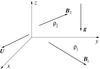 |
Fig. 1 Sketch of the equilibrium. |
2. Problem formulation
We considered the Rayleigh-Taylor instability of a magnetic tangential discontinuity in the presence of a plasma flow. We assumed that the equilibrium magnetic field is sheared, meaning that it has different directions at the two sides of the discontinuity. We used the reference frame where the plasma with lower density is at rest (see Fig. 1). In what follows, we use Cartesian coordinates x,y,z with the z-axis antiparallel to the direction of the gravity acceleration. All equilibrium quantities but the plasma pressure p0 were assumed to be constant below (z< 0) and above (z> 0) the discontinuity, with the equilibrium density below the discontinuity lower than that above. The equilibrium plasma pressure is defined by the equation 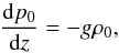 (1)where g is the gravity acceleration and ρ0 is the equilibrium plasma density.
The plasma motion is described by the linear ideal MHD equations for an incompressible plasma, 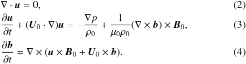 Here u is the perturbation of the plasma velocity, p the pressure perturbation, and b the magnetic field perturbation; B0 is the background magnetic field, U0 the background flow velocity, ρ0 the plasma density, and μ0 the magnetic permeability of free space. The vectors B0 and U0 are parallel to the xy-plane. We have B0 = B1, U0 = 0, and ρ0 = ρ1 for z< 0, and B0 = B2, U0 = U, and ρ0 = ρ2 for z> 0. In what follows we assume that ρ1<ρ2.
Equations (2)–(4) have to be complemented with boundary conditions at z = 0. The first boundary condition is the kinematic condition. Writing the equation of the perturbed tangential discontinuity as z = η(t,x,y), we write this condition as  (5)where the subscripts 1 and 2 indicate that a quantity is calculated for z< 0 and z> 0, respectively. The second boundary condition is the dynamic boundary condition. It states that the total pressure, plasma plus magnetic, has to be continuous at the discontinuity. In the linearized form it reads
  (6)where the double brackets indicate the jump of a quantity across the discontinuity. To derive this boundary condition, we have used Eq. (1).
3. Solution of initial-value problem
In what follows we consider the perturbations that are independent of y. At the initial moment of time (t = 0), we impose the initial conditions  (7)We consider perturbations that decay as | x | + | z | → ∞. To solve the initial-value problem for the system of Eqs. (2)–(4) with the boundary conditions (5) and (6) and the initial conditions (7) we introduce the Fourier transform with respect to x,
  (8)and the Laplace transform with respect to time,
  (9)Here σ is defined by the condition that the line ℑ(ω) = σ in the complex ω-plane is above all singularities of function
  , where ℑ indicates the imaginary part of a quantity.
We also introduce the notation  for the Laplace-Fourier transform of function f(t,x). Applying the Laplace-Fourier transform to Eqs. (2)–(4) and the boundary conditions (5) and (6), and using the initial conditions (7), we obtain
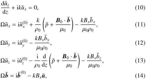
where Ω = ω − kUx, and Ux and Bx are the x-components of the equilibrium velocity and magnetic field respectively. The boundary conditions are transformed to
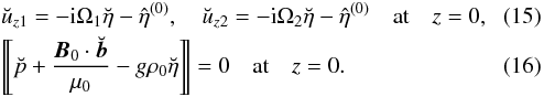 For the sake of simplicity, we assume below that the initial velocity perturbation is potential, ∇ × u(0) = 0, and the initial magnetic field perturbation is current free, ∇ × b(0) = 0. Then, eliminating all variables in Eqs. (10)–(14) in favor of uz, we obtain
 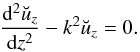 (17)The solution to this equation satisfying the boundary conditions (15) is
 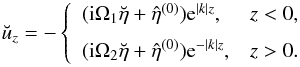 (18)Using Eqs. (10), (11) and (14) we obtain
 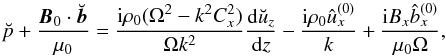 (19)where
  . With the aid of this expression we rewrite Eq. (16) as
 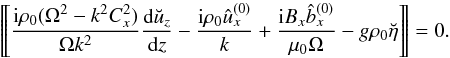 (20)Substituting Eq. (18) into this equation we obtain the expression for
  ,
,  (21)
(21)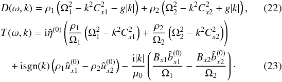 In this expression the quantities
  and
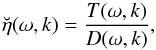
and  are calculated at z = 0. Now the function η(t,x) is given by
  (24)We see that the dispersion relation function, D(ω,k), represents the model, while the function T(ω,k) depends on the external perturbations and, hence, can be considered as arbitrary. In studying the stability with respect to normal modes as well as the absolute and convective instability, we only use the dispersion relation function D(ω,k) (e.g. Briggs 1964).
Studying the absolute and convective instabilities is based on using the analytical properties of function D(ω,k) considered as a function of two complex variables, ω and k. However, it is straightforward to see that D(ω,k) is not an analytical function of k because of the presence of | k | in Eq. (22). To overcome this difficulty, we note first of all that  for real k, where the long bar above a quantity indicates complex conjugate. Then, for real k, we have
  (25)Using these relations, we obtain
  (26)With the aid of this result, we transform Eq. (24) to
  (27)where
  (28)and ℜ indicates the real part of a quantity. Now we can use Eqs. (22) and (23) as defining functions T(ω,k) and D(ω,k) for positive k alone. In accordance with this we substitute k for | k | in the expressions for these functions. Now T(ω,k) and D(ω,k) are analytical functions of k, and we can extend them to the whole complex k-plane.
4. Normal modes
The dispersion equation for normal modes is D(ω,k) = 0. We introduce the dimensionless quantities 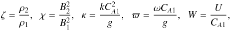 (29)where
  . We also introduce the angles α and β between U and B1, and U and B2, both angles being measured from U in the positive, that is counterclockwise direction (see Fig. 2). Finally, we introduce the angle ϕ between the positive x-direction and U, this angle being measured from the positive x-direction. In the dimensionless variables we rewrite the dispersion equation as
 ![\begin{eqnarray} \label{eq:4.2} (1 + \zeta)\varpi^2 &-& 2\kappa\varpi\zeta W\cos\varphi \nonumber\\ &&+ \kappa^2\big[\zeta W^2\cos^2\varphi - \Lambda(\varphi)\big] + (\zeta - 1)|\kappa| = 0 , \end{eqnarray}](/articles/aa/full_html/2015/08/aa25959-15/aa25959-15-eq84.png) (30)where
(30)where  (31)In what follows we impose the condition that there is no Kelvin-Helmholtz instability, that is the discontinuity is stable when g → 0. In this limit κ → ∞ and ϖ → ∞, while the ratio ϖ/κ remains finite.
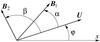 |
Fig. 2 Definition of angles. |
Hence, the condition that the discontinuity is stable when g → 0 reduces to the condition that the ϖ-roots of Eq. (30) are real when the last term on the right-hand side of this equation is dropped. This condition, in turn, reduces to 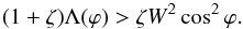 (32)This inequality can be rewritten as
 ![\begin{eqnarray} (1 \!&+&\! \zeta)(1 + \chi) - \zeta W^2 + \big[(1 + \zeta)(\cos2\alpha + \chi\cos2\beta) \nonumber\\ &&- \zeta W^2\big]\cos2\varphi > (1 + \zeta)(\sin2\alpha + \chi\sin2\beta)\sin2\varphi , \nonumber \end{eqnarray}](/articles/aa/full_html/2015/08/aa25959-15/aa25959-15-eq92.png) which can be further reduced to
which can be further reduced to  (33)where
 ![\begin{eqnarray} &&A^2 = (1 + \zeta)^2[1 + \chi^2 + 2\chi\cos(2\alpha - 2\beta)] + \zeta^2 W^4 \nonumber\\ \label{eq:4.5} &&\qquad- 2\zeta(1 + \zeta)W^2(\cos2\alpha + \chi\cos2\beta) , \\ \label{eq:4.6} &&\sin\psi = A^{-1}\big[(1+\zeta)(\cos2\alpha + \chi\cos2\beta) - \zeta W^2\big], \\ \label{eq:4.7} &&\cos\psi = A^{-1}(1 + \zeta)(\sin2\alpha + \chi\sin2\beta) , \end{eqnarray}](/articles/aa/full_html/2015/08/aa25959-15/aa25959-15-eq94.png) and A> 0. The inequality (33) must be satisfied for any direction of perturbation propagation, that is for any value of ϕ. Obviously its left-hand side takes its minimum at
and A> 0. The inequality (33) must be satisfied for any direction of perturbation propagation, that is for any value of ϕ. Obviously its left-hand side takes its minimum at  . Hence, the condition that the inequality (33) must be satisfied for any value of ϕ is
 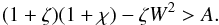 Using Eq. (34) we rewrite it as
  (37)In what follows we assume that this condition is satisfied.
The condition of the Rayleigh-Taylor instability is that the roots of Eq. (30) are complex. This condition is written as | κ | <κc(ϕ), where  (38)It follows from the inequality (32) that κc(ϕ) > 0. Equation (38) can be transformed to
  (39)It follows from this expression that κc(ϕ) takes its maximum at
  , and this maximum is given by
  (40)When | κ | <κc(ϕ), the roots of Eq. (30) can be written as ϖ = ϖr ± iϖi, where
 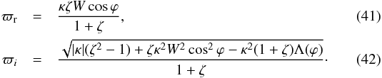 The quantity ϖi is the dimensionless instability increment. At fixed ϕ it takes its maximum, ϖim, at
  , where
  (43)The quantity ϖim considered as a function of ϕ takes its maximum at ϕ = ϕm. This maximum is given by
 ![\begin{equation} \max\varpi_{i{\rm m}} = \frac{\zeta - 1}{\sqrt{2\big[(1 + \zeta)(1 + \chi) - \zeta W^2 - A\big]}}\cdot \label{eq:4.16} \end{equation}](/articles/aa/full_html/2015/08/aa25959-15/aa25959-15-eq113.png) (44)When there is no flow (W = 0) all the results obtained in this section coincide with those obtained by Ruderman et al. (2014).
(44)When there is no flow (W = 0) all the results obtained in this section coincide with those obtained by Ruderman et al. (2014).
5. Absolute and convective instabilities
5.1. General analysis
To study the absolute and convective instabilities, we used the method developed by Briggs (1964; see also Bers 1973). In accordance with the results of the previous section D(ω,k) ≠ 0 for real k and ℑ(ω) >ωim. This implies that all k-roots of D(ω,k) = 0 are located away from the real k-axis when ℑ(ω) >ωim. Hence, in this region of the complex ω-plane, the function R(ω,x) is analytic, and we have to take σ>ωim. The contribution to the instability comes from singularities in the upper ω-plane of the analytic continuation of R(ω,x) from the above Bromwich integration contour ℑ(ω) = σ down to and slightly below the real ω-axis. The analytic continuation of the function R(ω,x) from above the Bromwich integration contour towards the real ω-axis is performed along the straight lines, as in the approach suggested by Briggs (1964; see also Bers 1973 and Brevdo 1988). We recall that D(ω,k) ≠ 0 for real k and ℑ(ω) >ωim. However, similar to the analysis in Ruderman et al. (2004), in the present case the function R(ω,x) is given by the integral from 0 to ∞, and not from −∞ to ∞ as was treated by Briggs (1964). This will introduce a modification into the procedure developed by Briggs (1964).
For a fixed ω0 with ℑ(ω0) ≥ 0, let ω ↘ ω0 denote the movement of ω down from ω to ω0 along a vertical straight line passing through ω0 (see Fig. 3a). For the analytic continuation of R(ω,x) we consider the movement of the two k-roots of D(ω,k) = 0 in the complex k-plane when ω ↘ ω0 (see Fig. 3b). If during the motion of ω towards ω0 one of the roots becomes real, then we have a singularity in the integrand in Eq. (28) that defines R(ω,x). However we can remove this singularity by deforming the integration contour in the complex k-plane, as is shown in Fig. 3b. The singularity cannot be removed only when the contour is pinched by the two k-roots that come from two different sides of the contour. We call a collision of roots on the deformed Fourier contour that causes its pinching a pinching collision. When no pinching collision of k-roots occurs as ω ↘ ω0, then the function R(ω,x) can be analytically continued along the vertical line as described above from the above the Bromwich integration contour down till ω = ω0 by appropriately deforming the Fourier integration contour in Eq. (28).
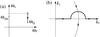 |
Fig. 3 a) Movement ω ↘ ω0 of ω. b) Trajectories of the k-roots of the dispersion equation D(ω,k) = 0 in the complex k-plane when ω ↘ ω0 (thin curves), the deformed Fourier integration contour (thick curve), and pinching of this contour by two k-roots |
If R(ω,x) can be analytically continued down and slightly below the real ω-axis, then the equilibrium is convectively unstable. It is absolutely unstable if the analytic continuation of R(ω,x) has singularities in the upper part of the complex ω-plane. At a point ω0 with ℑ(ω0) ≥ 0, for which a pinching collision of the two k-roots takes place, the function R(ω,x) has a branch point singularity of the form (ω − ω0)− 1/2 (Briggs 1964; Bers 1973; Brevdo 1988). Let, for ω = ω0, the pinching collision of the two k-roots takes place at k = k0. The dominant term of the contribution to the asymptotics of the expression for η(t,x) at fixed x and t → ∞ coming from this singularity has the form  (45)where the factor Q(ω0,k0) is independent of t and x.
A necessary condition for a pinching collision of the two k-roots is that, at the collision point (ω0,k0), the function D(ω,k) has a double root in k, that is,  (46)This condition, however, is not sufficient for pinching. In addition, it is necessary to verify that the two colliding k-roots come from different sides of the Fourier integration contour. As explained in Ruderman et al. (2004), this condition reduces to the following: consider the trajectories of the two k-roots obtained when ω ↘ ω0. Then the union of trajectories of the two roots has to cross the positive real k-axis odd number of times.
The analysis of absolute and convective instabilities is frame dependent: The equilibrium can be absolutely unstable in one reference frame and only convectively unstable in another. An analysis of the asymptotics of the solution in a reference frame moving with the velocity V ≠ 0 with respect to the reference frame where U0 = 0 for z< 0 can be performed in a similar way to the above analysis. In the moving reference frame the dispersion relation function is  . Hence, in this reference frame we use the system of equations
  (47)We recall that the expression for the function D(ω,k) is given by Eq. (28) with k substituted for | k |.
5.2. Calculations
We use the dimensionless variables defined by Eqs. (29) and the dimensionless reference frame velocity Υ = Vx/CA1 to write the system of Eqs. (47) in the dimensionless form: ![\begin{eqnarray} &&(1 + \zeta)(\varpi_0 + \kappa_0\Upsilon)^2 - 2\kappa_0(\varpi_0 + \kappa_0\Upsilon)\zeta W\cos\varphi \nonumber\\ \label{eq:5.4} &&\qquad\qquad\qquad +\, \kappa_0^2\big[\zeta W^2\cos^2\varphi - \Lambda(\varphi)\big] + (\zeta - 1)\kappa_0 = 0 ,\quad\quad \\ &&2\Upsilon(1 + \zeta)(\varpi_0 + \kappa_0\Upsilon) - 2(\varpi_0 + 2\Upsilon\kappa_0)\zeta W\cos\varphi \nonumber\\ \label{eq:5.5} &&\qquad\qquad\qquad +\, 2\kappa_0\big[\zeta W^2\cos^2\varphi - \Lambda(\varphi)\big] + \zeta - 1 = 0 . \end{eqnarray}](/articles/aa/full_html/2015/08/aa25959-15/aa25959-15-eq137.png) From the system of Eqs. (48) and (49) we obtain
From the system of Eqs. (48) and (49) we obtain 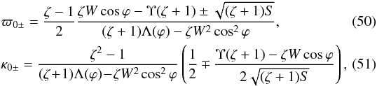 where
where  (52)The subscripts “+” or “−” in Eqs. (50) and (51) have to be the same.
If S ≥ 0, then ϖ0 is real and, in accordance with Eq. (45), the contribution from ϖ0 decays as t− 1/2. Hence, in this case, the instability is definitely convective. It can only be absolute if S< 0. In this case we put  . Since, in accordance with Eq. (32), the denominator in Eq. (50) is positive, it follows that ℑ(ϖ0 +) > 0 and ℑ(ϖ0 −) < 0, which means that the exponentially growing contribution can only come from ϖ0 +. In accordance with this below we put ϖ0 = ϖ0 + and κ0 = κ0 +. The condition S< 0 can be written as Υ−< Υ < Υ+, where
 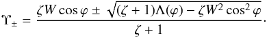 (53)The inequality (32) guaranties that Υ− and Υ+ are real.
As we have already pointed out, the condition ℑ(ϖ0) > 0 is insufficient for the instability to be absolute. We must also verify that the root κ0 is pinching. To do this we consider the trajectories of the κ-roots that are obtained when ω ↘ ω0. We put ϖ = ϖ0 + is, where s is a real non-negative variable. In Eq. (27) σ is any quantity satisfying σ>ϖim. Hence we can even take σ → ∞. This implies that we can take s ∈ [ 0,∞). Then the motion ω ↘ ω0 corresponds to decreasing s from infinity to zero. Now we write ϖ0 = ϖ0r + iϖ0i. Substituting κ for | κ | and ϖ0r + iϖ0i + is + κΥ for ϖ in the dispersion Eq. (30), we obtain ![\begin{eqnarray} (1 + \zeta)[\omega_{0r} &+& \kappa\Upsilon + i(\omega_{0i} + s)]^2 \nonumber\\ &-& 2\kappa\zeta W[\omega_{0r} + \kappa\Upsilon + i(\omega_{0i} + s)] \cos\varphi \nonumber\\ \label{eq:5.10} &+& \, \kappa^2\big[\zeta W^2\cos^2\varphi - \Lambda(\varphi)\big] + (\zeta - 1)\kappa = 0 . \end{eqnarray}](/articles/aa/full_html/2015/08/aa25959-15/aa25959-15-eq167.png) (54)We denote the two κ-roots of this equation as κ+(s) and κ−(s). It is straightforward to obtain the approximate solutions to Eq. (54) valid for s ≫ 1:
(54)We denote the two κ-roots of this equation as κ+(s) and κ−(s). It is straightforward to obtain the approximate solutions to Eq. (54) valid for s ≫ 1: 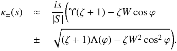 (55)Simple calculation shows that the inequality
  (56)is equivalent to Υ−< Υ < Υ+. This implies that ℑ [ κ−(s) ] < 0 and ℑ [ κ+(s) ] > 0, that is κ−(s) is in the lower and κ+(s) in the upper part of the complex plane when s ≫ 1.
Now we calculate a value of s corresponding to the intersection of the real axis by one of the κ-roots. To do this we assume that κ is real and take the real and imaginary part of Eq. (54). As a result we obtain the system of equations for κ and s: ![\begin{eqnarray} &&(1 + \zeta)\left[(\omega_{0r} + \kappa\Upsilon)^2 - (\omega_{0i} + s)^2\right] - 2\kappa\zeta W(\omega_{0r} + \kappa\Upsilon)\cos\varphi \nonumber\\ \label{eq:5.13} &&\qquad+\, \kappa^2\left[\zeta W^2\cos^2\varphi - \Lambda(\varphi)\right] + (\zeta - 1)\kappa = 0 , \\ \label{eq:5.14} &&(1 + \zeta)(\omega_{0r} + \kappa\Upsilon) - \kappa\zeta W\cos\varphi = 0 . \end{eqnarray}](/articles/aa/full_html/2015/08/aa25959-15/aa25959-15-eq175.png) When deriving Eq. (58) we have taken into account that ω0i + s> 0. The solution to the system of Eqs. (57) and (58) is straightforward, so we only present the final result:
When deriving Eq. (58) we have taken into account that ω0i + s> 0. The solution to the system of Eqs. (57) and (58) is straightforward, so we only present the final result: ![\begin{eqnarray} \label{eq:5.15} &&\kappa = \kappa_-(s_0) = \frac{\zeta^2 - 1}{2[(\zeta + 1)\Lambda(\varphi) - \zeta W^2\cos^2\varphi]} , \\ \label{eq:5.16} &&s_0 = \frac{(\zeta - 1)\big[\sqrt{(\zeta + 1)\Lambda(\varphi) - \zeta W^2\cos^2\varphi} + \sqrt{(\zeta + 1)|S}|\big]} {2[\Upsilon(\zeta + 1) - \zeta W\cos\varphi]^2 [(\zeta + 1)\Lambda(\varphi) - \zeta W^2\cos^2\varphi]} \cdot\quad\quad \end{eqnarray}](/articles/aa/full_html/2015/08/aa25959-15/aa25959-15-eq177.png) It follows from Eq. (32) that s0> 0 and κ−(s0) > 0. We can be sure that it is κ−(s) that crosses the real axis because ℑ [ κ−(s) ] < 0 when s ≫ 1, while κ−(0) = κ0 and ℑ(κ0) > 0. We see that the union of trajectories of the two roots crosses the real k-axis just once, that is, odd number of times. This implies that k0 is the pinching root, and the condition Υ−< Υ < Υ+ is necessary and sufficient for the instability to be absolute.
It follows from Eq. (32) that s0> 0 and κ−(s0) > 0. We can be sure that it is κ−(s) that crosses the real axis because ℑ [ κ−(s) ] < 0 when s ≫ 1, while κ−(0) = κ0 and ℑ(κ0) > 0. We see that the union of trajectories of the two roots crosses the real k-axis just once, that is, odd number of times. This implies that k0 is the pinching root, and the condition Υ−< Υ < Υ+ is necessary and sufficient for the instability to be absolute.
When Υ ∉ (Υ−,Υ+), the initial perturbation propagating in the direction defined by the angle ϕ will decay at any fixed spatial position. Perturbations propagating in any direction will decay at any fixed spatial position only if | Υ | > Υ∗, where  (61)When deriving this result we have used an obvious identity Υ−(π − ϕ) = −Υ+(ϕ). The calculation of Υ∗ reduces to the solution of a quartic equation. In principle, it is hence possible to give the analytical expression for Υ∗. However, this expression is so complicated that it cannot be used in any application. It is much simpler to calculate Υ∗ numerically for any given value of parameters. We only give the estimate
  (62)The condition | Υ | > Υ∗ is sufficient for the instability to be convective, but it is not necessary.
On the bases of these results, we can make one important conclusion. In the reference frame where the plasma in the lower half-space (z< 0) is at rest (Υ = 0) there is always such a value of ϕ that the perturbation propagating at this angle is absolutely unstable.
6. Application to oscillating threads
Ruderman et al. (2014) used the results of studying the MRT instability to estimate the angle between the magnetic field inside a prominence thread and in the external plasma. Their analysis was based on the observation of oscillating thread reported by Okamoto et al. (2007). From the movie presented in this paper they estimated that the thread lifetime was about 10 min. Ruderman et al. (2014) assumed that the MRT instability is responsible for the short lifetime of the thread and took this lifetime to be equal to the growth time of the most unstable mode.
It is difficult to make any conclusions about the presence of flow in the thread. Hence, it seems expedient to discuss a possible effect of flow on the estimate obtained by Ruderman et al. (2014). We assumed that there was a flow parallel to the magnetic field in the thread. In our notation this means that β = 0. We also assumed that there is no flow in the external plasma, therefore Υ = 0. In accordance with the conclusion made at the end of the previous section, there are always absolutely unstable perturbations propagating at particular angles with respect to the flow direction. In accordance with Eq. (45) the increment of the perturbation propagating at the angle ϕ is ℑ [ ϖ0(ϕ) ], where ϖ0(ϕ) is given by Eq. (50) with the “+” sign on the right-hand side (we recall that ℑ [ ϖ0(ϕ) ] ≠ 0 only when S< 0). The expression for the increment is now simplified to ![\begin{equation} \Im[\varpi_0(\varphi)] = \frac{(\zeta - 1)\sqrt{(\zeta + 1) \left[\cos^2(\varphi + \alpha) + \left(\chi - \zeta W^2\right)\cos^2\varphi\right]}} {2\left\{(\zeta + 1)\cos^2(\varphi + \alpha) + \left[\chi(\zeta + 1) - \zeta W^2\right]\cos^2\varphi\right\}}\cdot \label{eq:6.1} \end{equation}](/articles/aa/full_html/2015/08/aa25959-15/aa25959-15-eq194.png) (63)The inequality (37) that guarantees that there is no KH instability takes the form
(63)The inequality (37) that guarantees that there is no KH instability takes the form  (64)Note that ℑ [ ϖ0(ϕ) ] = ϖim when W = 0, that is, in the absence of flow, the growth rate of the wave packets propagating in the ϕ-direction is the same as the growth rate of the most unstable normal mode. This is an expected result (see, e.g. Briggs 1964) because, in accordance with Eq. (41), the real part of the frequency of a normal mode is zero when W = 0.
Similar to Ruderman et al. (2014), we assumed that ζ ≫ 1, α ≪ 1, and χ ~ 1. Then we can use the approximations sinα ≈ α and  . Since we only consider unstable perturbations, the expression under the square root in Eq. (63) must be positive. This implies that ζW2< 1 + χ. Then ζW2 ≪ χ(ζ + 1), and we can neglect the term proportional to W2 in the denominator on the right-hand side of Eq. (64). As a result, we obtain the approximate expression for the increment,
 ![\begin{equation} \Im[\varpi_0(\varphi)] \approx \frac{\sqrt{\zeta\left[(1 + \chi - \zeta W^2) \cos^2\varphi - \alpha\sin2\varphi - \alpha^2\cos2\varphi\right]}} {2\left[(1 + \chi)\cos^2\varphi - \alpha\sin2\varphi - \alpha^2\cos2\varphi\right]}\cdot \label{eq:6.3} \end{equation}](/articles/aa/full_html/2015/08/aa25959-15/aa25959-15-eq205.png) (65)To calculate the maximum value of ℑ [ ϖ0(ϕ) ], we note that when ϕ is not close to either π/ 2 or 3π/ 2, the denominator is on the order of unity, while the numerator is on the order or
(65)To calculate the maximum value of ℑ [ ϖ0(ϕ) ], we note that when ϕ is not close to either π/ 2 or 3π/ 2, the denominator is on the order of unity, while the numerator is on the order or  . Hence, ℑ [ ϖ0(ϕ) ] is on the order of . On the other hand, when the difference between ϕ and either π/ 2 or 3π/ 2 is on the order of α, the denominator is on the order of α2, while the numerator is on the order or
  . Hence, ℑ [ ϖ0(ϕ) ] is on the order of
  . This analysis shows that when looking for the maximum value of ℑ [ ϖ0(ϕ) ], we can assume that ϕ is close to either π/ 2 or 3π/ 2. In addition, noticing that ℑ [ ϖ0(ϕ) ] is a periodic function of ϕ with the period π, we can consider ϕ close to π/ 2 only. Therefore we put ϕ = π/2 − ψ and assume that | ψ | ≪ 1. Then Eq. (65) reduces to
 ![\begin{equation} \Im[\varpi_0(\varphi)] \approx \frac{M\sqrt\zeta}{2\alpha}, \quad M = \frac{\sqrt{(1 + \chi - \zeta W^2)r^2 - 2r + 1}} {(1 + \chi)r^2 - 2r + 1}, \label{eq:6.4} \end{equation}](/articles/aa/full_html/2015/08/aa25959-15/aa25959-15-eq215.png) (66)where r = ψ/α. When W = 0 the calculation of maxℑ [ ϖ0(ϕ) ] is straightforward and we obtain
(66)where r = ψ/α. When W = 0 the calculation of maxℑ [ ϖ0(ϕ) ] is straightforward and we obtain  . When W ≠ 0, calculating Mm reduces to solving a cubic equation. Hence, in principle, it is possible to give the analytical expression for Mm. However, this expression is so complicated that it cannot be used in any application. It is much more practical to calculate it numerically. In Fig. 4 the dependence of Mm on the parameter
  is shown for χ = 1. We note that in this case
  , where
  . In accordance with the restriction ζW2< 1 + χ, the dimensionless flow magnitude U/CA2 varies from 0 till
  . It can be seen that Mm and, consequently, maxℑ [ ϖ0(ϕ) ] is a monotonically decreasing function of the parameter . In fact, this is a general result valid for any χ. Using Eq. (63) it is easy to show that ℑ [ ϖ0(ϕ) ] is a monotonically decreasing function of the parameter at any fixed ϕ. It follows from this result that maxℑ [ ϖ0(ϕ) ] is also a monotonically decreasing function of the parameter . This result has a simple physical explanation. Although the flow cannot completely wipe out the perturbations from any finite spatial domain and make the instability convective, it still wipes out the perturbations partially and thus reduces the growth rate.
For the growth time of the fastest growing perturbation, τg, which is the inverse to the maximum instability increment, we obtain  (67)When χ = 1 and W = 0, this result coincides with a similar result obtained by Ruderman et al. (2014, see Eq. (57) in that paper).
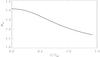 |
Fig. 4 Dependence of Mm on the flow magnitude. |
Ruderman et al. (2014) assumed that the lifetime of the thread is equal to the growth time of the MRT instability. Then, using the relation between τg and α, they estimated α. The gravity acceleration at the solar surface is g = 274 m/s2 (Priest 1982). In their calculations, Ruderman et al. (2014) took χ = 1 and CA2 = 500 km s-1, and obtained α ≈ 13°. It is seen in Fig. 4 that the dependence of Mm on U/CA2 is quite week. When U/CA2 varies from 0 till its maximum value , Mm decreases from  to 1.14. This implies that the presence of flow has little effect on the estimate of the angle α. Even if we assume that the flow magnitude in the thread is equal to its maximum possible value
  km s-1, which is unrealistically high, then the estimate for α will be reduced from 13° to 10.5°.
7. Application to the heliopause stability
In this section we apply the results obtained in the previous sections to the heliopause stability. As we explained in Sect. 2, the heliopause separates the solar wind, decelerated at the termination shock, and the interstellar medium flow, decelerated at the bow shock (see the schematic of the heliosphere shown in Fig. 5). Obviously, the heliopause is a transitional region of finite thickness. It can only be treated as a tangential discontinuity when we consider perturbations with a wavelength much larger than its thickness. At present, there are no observational data that enable estimating the heliopause thickness. We restrict our analysis to perturbations with a characteristic wavelength much smaller than the curvature radius of the heliopause at the apex point, but much larger than (that at present unknown) heliopause thickness. Then, at the distances from the apex point much larger than the perturbation characteristic wavelength, we can carry out the local stability analysis and consider the heliopause as a planar tangential discontinuity. Following to Ruderman et al. (2004), we also only consider the near flanks of the heliopause only (θ ≲ 30°). In this region, the plasma flow near the heliopause is strongly subsonic, meaning that the plasma flow can be considered as approximately incompressible.
However, the fact that the plasma flow is strongly subsonic does not guarantee that we can use the approximation of incompressible plasma when studying the RT instability. While the condition for the onset of the RT instability in an incompressible medium is g·∇ρ0< 0, this condition for a compressible gas reads g·∇s0> 0 with an assumption that the wavelength is much shorter than the pressure scale length, | p0(∂p0/∂x)-1 | (Bateman 1978). Here,  is the specific entropy, and γ = 5/3 is the ratio of specific heats. The assumption that the wavelength is much shorter than the pressure scale length is definitely satisfied for perturbations whose length is much smaller that the heliopause curvature radius because | p0(∂p0/∂x)-1 | is on the order of the heliosheath thickness which, in turn, is on the order of the heliopause curvature radius. We have
  . The ratio of the first term to the second term in this expression is on the order of the ratio of the heliopause thickness to the heliosheath thickness, which is much smaller than one. Hence, we can take
  , and the condition g·∇s0> 0 reduces to g·∇ρ0< 0. This result implies that we can use the approximation of an incompressible medium when studying the RT instability of the heliopause.
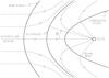 |
Fig. 5 Schematic of the heliosphere. |
Since the solar wind magnetic field is almost parallel to the termination shock, its direction after the shock is almost the same as before the shock, and only its magnitude increases. Hence, we can expect that it is still sufficiently well described by the Parker spiral (Parker 1958, 1963) in the inner heliosheath. It should therefore be parallel to the plasma flow velocity near the heliopause. On the other hand, there is evidence that the interstellar magnetic field is tilted (e.g. Opher et al. 2009) with an angle between the plasma flow and the field of between 20° and 30°. For the magnetic field magnitude, we used the observational results obtained by Voyager 1 and reported by Burlaga & Ness (2014). The observed magnetic field was strongly fluctuating, but we can take as typical values B1 = 0.2 nT and B2 = 0.4 nT, where now the indices 1 and 2 refer to the inner and outer heliosheath. Hence, χ = 4. The direction of the flow velocity at the two sides of the heliopause is approximately the same and we obtain α = 0, while β is between 20° and 30°.
Below we also need the values of the plasma densities and flow velocities at the two sides of the heliopause. We took these values from a long-known article by Baranov et al. (1979). In the 35 yr that passed after the publication of this article, the model of the interaction between solar wind and interstellar medium was greatly advanced. However, the values and variation of the plasma density and velocity along the heliopause remain qualitatively the same. On the other hand, the article by Baranov et al. (1979) has the advantage that it presents the variation of the velocity and density along the heliopause in a very clear graphical form. In view of the great uncertainty in the magnetic field parameters, it seems possible to use the values given in Baranov et al. (1979) for our qualitative MRT instability model.
Taking into account that the flow near the heliopause can be considered as plane parallel only sufficiently far from the stagnation point, we restricted our analysis to 10° ≤ θ ≤ 30°. For these values of θ, the plasma density at the two sides of the heliopause is almost constant. We took the electron concentration in the interstellar medium to be equal to 4 × 10⁴ m-3. Since the bow shock is weak (some authors even argue that it does not exist at all, e.g. McComas et al. 2012), we took the same value for the electron concentration at the heliopause. Then we obtain ρ2 ≈ 6.7 × 10⁻²³ kg m-3. We also took the ratio of densities at the two sides of the heliopause equal to ζ = ρ2/ρ1 = 50. Then we obtain CA1 ≈ 154 km s-1 and CA2 ≈ 44 km s-1. Estimates show that the plasma beta at both sides of the heliopause is on the order of unity. Hence, although it is desirable to account for compressibility in studying the MRT instability of the heliopause, we do not expect that it can substantially change the results of the analysis.
We also took the interstellar medium velocity to be equal to 20 km s-1 and the solar wind velocity at the termination shock equal to 400 km s-1. Then we used the results given in Baranov et al. (1979) that the plasma velocity at the solar wind side of the heliopause, | U1 |, increases approximately from 26 km s-1 to 83 km s-1, and the plasma velocity at the interstellar medium side of the heliopause, | U2 |, increases approximately from 2 km s-1 to 6 km s-1 when θ increases from 10° to 30°. To have U> 0 we chose the x-axis in the direction of θ decrease, so both U1 and U2 are negative. Then we obtained for the dimensionless parameters W = (|U1 | − | U2|) /CA1 = 0.156 ÷ 0.5 and Υ = | U1 | /CA1 = 0.17 ÷ 0.54.
When α = 0, the condition that there is no KH instability given by Eq. (37) takes a very simple form: ζW2< 1 + ζ. Since W ≤ 0.5, this condition is satisfied with a very good margin. However, an MRT instability is possible. When the solar wind dynamic pressure increases, the heliospheath is accelerated toward the interstellar medium. This acceleration can act as an effective gravitation in the non-inertial reference frame where the heliospheath is at rest. Υ+(0) is a monotonically decreasing function of β. Simple calculation gives that, even for the maximum value of β = 30°, Υ+(0) increases from 0.43 to 0.76 when θ increases from 10° to 30°, and for any θ ∈ [ 10°,30° ] we have | Υ | < Υ+(0). Since Υ∗ ≥ Υ+(0), it follows that | Υ | < Υ∗. This result implies that the perturbations are absolutely unstable for at least some propagation angles. In particular, the perturbations propagating in the anti-flow direction are absolutely unstable. Consequently, the near flanks of the heliopause are absolutely unstable with respect to the MRT instability.
8. Summary and conclusions
We studied the magnetic Rayleigh-Taylor (MRT) instability of a magnetohydrodynamic tangential discontinuity in an infinitely conducting incompressible plasma in the presence of flow. We have assumed that the flow magnitude is small enough to guarantee that there is no Kelvin-Helmholtz (KH) instability. The normal mode analysis showed that perturbations with any wavelength are unstable when the magnetic field has the same direction at both sides of the discontinuity. As a result, the perturbation growth rate is unbounded and the initial-value problem describing the evolution of perturbations is ill posed. However, when there is the magnetic shear, only the perturbations whose wavelength is greater than the critical one are unstable. As a consequence, the perturbation growth rate is bounded and the initial-value problem is well posed.
We also studied the absolute and convective nature of the MRT instability. To do this we solved the initial-value problem using the Fourier transform with respect to the spatial variable and the Laplace transform with respect to time. Then we used the Briggs method. We obtained the necessary and sufficient condition for a perturbation propagating in a given direction to be only convectively unstable but absolutely stable. We also obtained the condition for perturbations propagating in any direction to be only convectively unstable but absolutely stable.
The results of the general analysis were applied to the MRT instability of prominence threads and the heliopause. Similar to Ruderman et al. (2014), we assumed that the thread disappearance is related to the MRT instability and the thread lifetime is equal to the inverse instability increment. Using this assumption, Ruderman et al. (2014) estimated the angle α between the magnetic field inside the thread and in the surrounding plasma. We assumed that there is a plasma flow inside the thread and studied how the magnitude of this flow affects the estimate of α. We found that the effect is very weak.
To apply this to the heliopause stability we carried out the local analysis and restricted it to the near flanks of the heliopause only where the plasma flow can be considered incompressible. We showed that there is no KH instability for values of the magnetic field magnitude observed by Voyager 1 and reported by Burlaga & Ness (2014). We then studied the MRT stability that can occur when the heliosheath is accelerated in the antisolar direction due to the increase in the solar wind dynamic pressure. This acceleration can act as an effective gravitation. We showed that, for typical values of the plasma flow and magnetic field parameters, there are directions such that perturbations propagating in these directions are absolutely unstable.
We finally add the following comment: we studied the absolute and convective instabilities of perturbations that have the form of plane waves. This means that they are invariant in the spatial direction that is parallel to the discontinuity and orthogonal to the propagation direction. Hence, the perturbations occupy a domain that is finite in the propagation direction but infinite in the orthogonal direction. For the sake of brevity, we call these the perturbations of the first kind. In reality, any perturbation has to occupy a spatial domain bounded in both directions. Again for the sake of brevity, we call these the perturbations of the second kind. Obviously, if perturbations of the first kind propagating in any direction are only convectively unstable but absolutely stable, then the same is true for the perturbations of the second kind. However, it is possible that all perturbations of the second kind are only convectively unstable, but absolutely stable even if perturbations of the first kind propagating in some directions are absolutely unstable.
References
- Baranov, V. B. 2009a, Space Sci. Rev., 143, 449 [NASA ADS] [CrossRef] [Google Scholar]
- Baranov, V. B. 2009b, Space Sci. Rev., 142, 23 [NASA ADS] [CrossRef] [Google Scholar]
- Baranov, V. B., Krasnobaev, K. V., & Kulikovskii, A. G. 1971, Sov. Phys. Dokl., 15, 791 [NASA ADS] [Google Scholar]
- Baranov, V. B., Lebedev, M. G., & Ruderman, M. S. 1979, Astrophys. Space Sci., 66, 441 [NASA ADS] [CrossRef] [Google Scholar]
- Baranov, V. B., Fahr, H. J., & Ruderman, M. S. 1992, A&A, 261, 341 [NASA ADS] [Google Scholar]
- Bateman, G. 1978, MHD instability (Cambridge, Mass: MIT Press) [Google Scholar]
- Bers, A. 1973, Theory of absolute and convective instabilities, Survey Lectures, Proc. Int. Congr. Waves and Instabilities in Plasmas, eds. G. Auer, & F. Cap, Institute for Theoretical Physics, Austria, 1 [Google Scholar]
- Brevdo, L. 1988, Geophys. Astrophys. Fluid Dynam., 40, 1 [NASA ADS] [CrossRef] [Google Scholar]
- Briggs, R. J. 1964, Electron-stream interaction with plasmas (Cambridge, MA: MIT Press) [Google Scholar]
- Bucciantini, N., Amato, E., Bandiera, R., Blondin, J. M., & Del Zanna, L. 2004, A&A, 423, 253 [NASA ADS] [CrossRef] [EDP Sciences] [Google Scholar]
- Burlaga, L. F., & Ness, N. F. 2014, ApJ, 784, 146 [NASA ADS] [CrossRef] [Google Scholar]
- Díaz, A. J., Soler, R., & Ballester, J. L. 2012, ApJ, 754, 41 [NASA ADS] [CrossRef] [Google Scholar]
- Díaz, A. J., Khomenko, E., & Collados, M. 2014, A&A, 564, A97 [NASA ADS] [CrossRef] [EDP Sciences] [Google Scholar]
- Fahr, H. J., Neutsch, W., Grzedzielski, S., Macek, W., & Ratkiewicz-Landowska, R. 1986, Space Sci. Rev., 43, 329 [NASA ADS] [CrossRef] [Google Scholar]
- Isobe, H., Miyagoshi, T., Shibata, K., & Yokoyama, T. 2005, Nature, 434, 478 [NASA ADS] [CrossRef] [Google Scholar]
- Isobe, H., Miyagoshi, T., Shibata, K., & Yokoyama, T. 2006, PASJ, 58, 423 [Google Scholar]
- Jun, B.-I., Norman, M. L., & Stone, J. M. 1995, ApJ, 453, 332 [NASA ADS] [CrossRef] [Google Scholar]
- McComas, D. J., Alexashov, D., Bzowski, M., et al. 2012, Science, 336, 1291 [NASA ADS] [CrossRef] [Google Scholar]
- Mills, K. J., Longbottom, A. W., Wright, A. N., & Ruderman, M. S. 2000, J. Geophys. Res., 105, 27685 [NASA ADS] [CrossRef] [Google Scholar]
- Okamoto, T. J., Tsuneta, S., Berger, T. E., et al. 2007, Science, 318, 1577 [NASA ADS] [CrossRef] [PubMed] [Google Scholar]
- Opher, M., Alouani Bibi, F., Toth, J., et al. 2009, Nature, 462, 1036 [NASA ADS] [CrossRef] [PubMed] [Google Scholar]
- Parker, E. N. 1958, ApJ, 128, 664 [Google Scholar]
- Parker, E. N. 1963, Interplanetary dynamical processes (New York: Interscience Publishers) [Google Scholar]
- Priest, E. 1982, Solar Magneto-Hydrodynamics, Geophysics and Astrophysics Monographs (Kluwer Academic Publishers) [Google Scholar]
- Ruderman, M. S. 2000, Astrophys. Space Sci., 274, 327 [Google Scholar]
- Ruderman, M. S., & Belov, N. A. 2010, J. Phys.: Conf. Ser., 216, 012016 [Google Scholar]
- Ruderman, M. S., & Fahr, H. J. 1993, A&A, 275, 635 [NASA ADS] [Google Scholar]
- Ruderman, M. S., & Fahr, H. J. 1995, A&A, 299, 258 [NASA ADS] [Google Scholar]
- Ruderman, M. S., Brevdo, L., & Erdélyi, R. 2004, Proc. R. Soc. Lond. A, 460, 847 [NASA ADS] [CrossRef] [Google Scholar]
- Ruderman, M. S., Terradas, J., & Ballester, J. L. 2014, ApJ, 785, A110 [NASA ADS] [CrossRef] [Google Scholar]
- Ryutova, M. P., Berger, T., Frank, Z., Tarbell, T., & Title, A. 2010, Sol. Phys., 267, 75 [Google Scholar]
- Stone, J. M., & Gardiner, T. 2007, ApJ, 671, 1696 [Google Scholar]
- Taroyan, Y., & Ruderman, M. S. 2011, Space Sci. Rev., 158, 505 [NASA ADS] [CrossRef] [Google Scholar]
- Terradas, J., Oliver, R., & Ballester, J. L. 2012, A&A, 541, A102 [NASA ADS] [CrossRef] [EDP Sciences] [Google Scholar]
- Wright, K. J., Mills, K. J., Ruderman, M. S., & Brevdo, L. 2000, J. Geophys. Res., 105, 385 [NASA ADS] [CrossRef] [Google Scholar]
- Wright, K. J., Mills, K. J., Longbottom, A. W., & Ruderman, M. S. 2002, J. Geophys. Res., 107, 1242 [CrossRef] [Google Scholar]
All Figures
|
Fig. 1 Sketch of the equilibrium. |
| In the text | |
|
Fig. 2 Definition of angles. |
| In the text | |
|
Fig. 3 a) Movement ω ↘ ω0 of ω. b) Trajectories of the k-roots of the dispersion equation D(ω,k) = 0 in the complex k-plane when ω ↘ ω0 (thin curves), the deformed Fourier integration contour (thick curve), and pinching of this contour by two k-roots |
| In the text | |
|
Fig. 4 Dependence of Mm on the flow magnitude. |
| In the text | |
|
Fig. 5 Schematic of the heliosphere. |
| In the text | |
Current usage metrics show cumulative count of Article Views (full-text article views including HTML views, PDF and ePub downloads, according to the available data) and Abstracts Views on Vision4Press platform.
Data correspond to usage on the plateform after 2015. The current usage metrics is available 48-96 hours after online publication and is updated daily on week days.
Initial download of the metrics may take a while.