| Issue |
A&A
Volume 580, August 2015
|
|
|---|---|---|
| Article Number | A111 | |
| Number of page(s) | 9 | |
| Section | Galactic structure, stellar clusters and populations | |
| DOI | https://doi.org/10.1051/0004-6361/201425577 | |
| Published online | 11 August 2015 | |
The nature of the KFR08 stellar stream
A chemical tagging experiment⋆
Lund ObservatoryDepartment of Astronomy and Theoretical
Physics,
Box 43,
221 00
Lund,
Sweden
e-mail: cheng@astro.lu.se; sofia@astro.lu.se; greg@astro.lu.se
Received: 23 December 2014
Accepted: 24 June 2015
The origin of the new kinematically identified metal-poor stellar stream, the KFR08 stream, has not been established to date. We present stellar parameters, stellar ages, and detailed elemental abundances for Na, Mg, Al, Si, Ca, Sc, Ti, Cr, Ni, Zn, Sr, Y, Zr, Ba, La, and Eu for 16 KFR08 stream members based on an analysis of high-resolution spectra. Based on the abundance ratios of 14 elements, we use the chemical tagging method to identify the stars with the same chemical composition that therefore might have a common birthplace, such as a cluster. Although three stars were tagged with similar elemental abundances ratios, we find that, statistically, it is not certain that they originate from a dissolved star cluster. This conclusion is consistent with the large dispersion of [Fe/H] (σ[ Fe / H ] = 0.29) among the 16 stream members. We find that our stars are α enhanced and that the abundance patterns of the stream members match the thick-disc population well. In addition, most of the stream stars have estimated stellar ages greater than 11 Gyr. These results, together with the hot kinematics of the stream stars, suggest that the KFR08 stream originated from the thick-disc population, which was perturbed by a massive merger in the early Universe.
Key words: Galaxy: evolution / Galaxy: formation / Galaxy: disk / solar neighborhood / stars: abundances / stars: kinematics and dynamics
© ESO, 2015
1. Introduction
Stellar streams, which are groups of stars that are on the same orbit in the Galactic potential, have been detected as over-densities in the velocity distribution of stars in the solar neighbourhood (e.g., Dehnen 1998; Famaey et al. 2005; Arifyanto & Fuchs 2006). Helmi et al. (1999) discovered the signature of a cold stream in the velocity distribution of the halo and interpreted this stream as part of the tidal debris of a disrupted satellite galaxy accreted by the Milky Way. Moreover, several studies (Navarro et al. 2004; Helmi et al. 2006; Arifyanto & Fuchs 2006) have concluded that the Arcturus stream is another such debris stream dating back to an accretion event 5 to 8 Gyr ago. The external origin of these halo streams is supported by numerical simulations (Helmi et al. 2003) and observations of ongoing satellite accretion such as that of the Sagittarius dwarf galaxy (Ibata et al. 1994).
However, accreted satellites are not the only source of streams. A stellar stream that is homogenous in age and chemical composition is associated with a dissolved star cluster. One striking example is the HR 1614 stream (Eggen 1978; Feltzing & Holmberg 2000; De Silva et al. 2007b). Stellar streams can also originate from dynamical effects within the discs that are due to resonances with the bars or spiral arms (Dehnen 2000; Antoja et al. 2009). Analysis of high-resolution spectra of nearby F and G dwarf stars has revealed that the stars in the Hercules stream have a wide range of stellar ages, metallicities, and element abundances (Bensby et al. 2007). Bensby and collaborators concluded that the kinematical properties of the Hercules stream are coupled to dynamical interactions with the Galactic bar.
Stellar parameters of KFR08 stream members.
Galactic coordinates, distances, space velocities, radial velocities, masses, absolute magnitudes, and ages of KFR08 stream members.
A new candidate stream, called the KFR08 stream, was recently discovered on a quite radial orbit by Klement et al. (2008) when they studied the RAVE data release (DR) 1 experimental data (Steinmetz et al. 2006). This stream is present as a broad feature in the range − 180 km s-1 ≤ V ≤ −140 km s-1 centred on V ≈ −160 km s-1 and would belong to the stellar halo population. The velocities, including U and W, here are given relative to the local standard of rest (LSR). Because of the high W-velocities of the stars in the stream, an origin external to the Milky Way’s disc was suggested by Klement et al. (2008). This was supported by Klement et al. (2009) and Bobylev et al. (2010) from analysing two independent data sets. Klement et al. (2009) characterized the orbits of calibrated stars from SDSS DR7 data (Abazajian et al. 2009) through angular momentum, eccentricity, and orbital polar angle. An over-density region that corresponds to the location of the KFR08 stream within parameter distributions was found. Based on a new version of the Hipparcos catalogue (van Leeuwen 2007) and updated Geneva-Copenhagen Survey (Holmberg et al. 2007) of F and G dwarfs, Bobylev et al. (2010) identified statistically significant signals of the main inhomogeneities in the velocity distribution using the wavelet transform technique. They found 19 possible stream members around (–160, 225) km s-1 in the V and (U2 + 2V2)1 / 2 plane. However, the KFR08 stream could not be completely confirmed by re-analysing the pure RAVE DR2 dwarf sample (Klement et al. 2011). At the phase-space position of the KFR08 stream, five stars identified from DR2 have a large scatter in metallicity. This is inconsistent with the prediction of chemical homogeneity of stream members if they come from a single cluster. But it might agree with the idea proposed by Minchev et al. (2009) that this high-velocity stream has a dynamical origin in the thick disc. It is thought to arise due to a sudden energy kick imposed by a massive satellite in the past. The signature of this perturbation can be identified in the stellar kinematics if it was not wiped out by the radial mixing (see Bland-Hawthorn et al. 2010) within the thick disc.
Although brilliant works on dynamical analysis have been done, the detailed elemental abundance and age structure of the KFR08 stream have never been investigated. Analysis of high-resolution spectra of possible stream members could give us more clues for exploring the origin of the stream. We here report on selecting candidates of the stream from databases and observing their spectra using different instruments in Sect. 2. We determine stellar parameters, ages, and elemental abundances from the spectra in Sect. 3. In Sect. 4, we use chemical tagging to identify the putative cluster stars from the kinematically detected KFR08 stream. The possible origins of the stream are discussed in Sect. 5. Finally, conclusions are drawn in Sect. 6.
2. Observations
2.1. Stellar sample
Bobylev et al. (2010) found nineteen stars that probably are members of the KFR08 stream. Seventeen of those are high-probability members. For 16 of them we analysed high-resolution spectra. These stars and their properties are listed in Table 1. We also give their Galactic coordinates, distances to the Sun, and space velocities with respect to the LSR in Table 2.
2.2. Spectroscopic observations
FIES observation.
Observations were carried out at the Nordic Optical Telescope (NOT) for ten of the candidates using the fibre-fed Echelle Spectrograph (FIES) on January 10–12, 2012. A solar spectrum was also obtained by observing the sky at daytime. The wavelength range of the spectra is 370–730 nm, with a resolving power R ~ 67 000, and the average signal-to-noise ratio (S/N) is higher than 100 per pixel for most of the spectra. All the spectra were reduced using the FIEStool1 pipeline. The pipeline includes the following steps to reduce the observed frame: subtracting bias and scattered light, dividing by a normalized two-dimensional flat field, extracting individual orders, and solving wavelength. Finally, all individual spectral orders are merged into a 1D spectrum.
Archival data.
Reduced 1D spectra for six stars were extracted from the ESO archive. We found that three stars have been observed using the UVES spectrograph (Dekker et al. 2000) on the VLT 8 m telescope in 2013. Two spectra have a medium resolution of R ~ 45 000, while the spectrum of star HIP 59785 was obtained in high-resolution mode (R ~ 110 000). The S/N values of these three spectra are higher than 100 per rebinned pixel. The spectrum for HIP 117702 was observed in 2006 with FEROS on the ESO 2.2 m telescope (Kaufer et al. 1999). This spectrum has a wide wavelength range (350–920 nm), high resolution (R ~ 48 000), and good S/N (~ 75 per rebined pixel). The exoplanet survey carried out with HARPS on nearby stars with high-resolution spectroscopy (R ~ 120 000, Mayor et al. 2003) includes spectra for two of the stars identified as possible stream members by Bobylev et al. (2010). Both spectra have a mean S/N higher than 50 per rebinned pixel.
Radial velocities (RVs) were measured by cross-correlating the solar synthesis spectrum with the observed spectra, making use of the packages RVSAO and XCSAO within IRAF2. Both our own spectra and collected spectra from the archive were shifted to rest wavelength by cross-correlation with a synthetic solar spectrum using the IRAF task DOPCO.
3. Abundance analysis
3.1. Stellar parameters
For our spectral analysis, we used Spectroscopy Made Easy (SME, Valenti & Piskunov 1996; Valenti & Fischer 2005) to determine both stellar parameters and elemental abundances by comparing synthetic spectra with observations. In SME the model atmospheres are interpolated in the precomputed MARCS model atmosphere grid (Gustafsson et al. 2008), which have standard composition.
The stellar parameters (Teff, log g, [Fe/H]) were determined following the same methodology as Liu et al. (2015, hereafter L15). We refer to L15 for full details. In brief, the initial stellar parameters that were used to generate a synthetic spectrum were estimated before running SME. As most of the candidates have metallicities around –0.7 dex (Table 2 in Bobylev et al. 2010), we assumed an initial [Fe/H] of –0.7 dex for all stars. Following the same methods as L15, initial effective temperatures (Teff) were determined using the colour-metallicity-temperature relations of Alonso et al. (1996), using both B − V and b − y colours, where B − V came from the Hipparcos catalogue (Perryman et al. 1997) and b − y values were obtained from the Strömgren survey (Olsen 1983, 1993; Schuster & Nissen 1988). An initial estimate of surface gravities (log g) were calculated using Teff, distances (from Hipparcos parallaxes), bolometric corrections, and stellar mass from the Yonsei-Yale isochrones (Demarque et al. 2004). Then, the stellar parameters (shown in Table 1) were determined by using a purely spectroscopic method (called Procedure 1 in L15). The location of stars in Teff vs. log g diagram are shown in Fig 1. Considering systematic errors and possible sources of uncertainty in the atmospheric model and atomic line data, the systematic uncertainties in the stellar parameters were estimated to be δTeff = 67 ± 40 K, δlog g = 0.08 ± 0.06 dex, and δ [ Fe / H ] = 0.06 ± 0.03 dex.
Since our stellar parameters are derived using Fe lines, which were compiled for the spectra of solar type stars, it is possible that the results may include systematic uncertainties due to departures from non-local thermodynamical equilibrium (NLTE, e.g., Bergemann et al. 2012). Following the same methodology as Ruchti et al. (2013), we derived stellar parameters for two stars (HIP 5336 and HIP 58708) using on-the-fly NLTE corrections for Fe. It was found that the mean differences between our results and stellar parameters determined from equivalent width method are ΔTeff = −67 K, Δlog g = 0.02 dex and Δ [Fe/H] = –0.02 dex, respectively. These differences are well within our estimated uncertainties and do not effect our chemical tagging experiment.
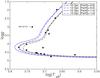 |
Fig. 1 Teff vs. log g diagram. Filled circles indicate our main sample from the Hipparcos catalogue. Isochrones at different ages (10 and 13 Gyr) and metallicities (–0.6 and –1.0 dex) according to the Yonsei-Yale models (Demarque et al. 2004) are shown. |
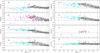 |
Fig. 2 Light elemental abundance ratios [X/Fe] as a function of [Fe/H]. Three tagged cluster stars (see Sect. 4) are indicated as red filled diamonds, while other stream stars are shown as black emptied diamonds. The disc stars from Bensby et al. (2014) are plotted as open gray circles, while the cyan triangles and magenta stars indicate the thick-disc and halo stars collected from Nissen & Schuster (2010) and Fulbright (2000), respectively. Dashed lines indicate solar values. |
As the precision of the parallax for all stars is better than 15%, based on the partly physical method (called Procedure 2 in L15), we also measured their stellar parameters (Table 1) by fixing log g as estimated from the Hipparcos parallaxes. Comparison with the log g estimated from the Fe lines, the differences between the two surface gravities are less than 0.15 dex for most of the stars. An exception was found for two stars, HIP 59785 and HIP 87101: their log g are changed by 0.6 dex. It was also found that the mean differences in Teff are larger than 200 K for these two stars. Since HIP 59785 is a very cool star with B − V> 1.0, we might overestimate log g from parallax caused by an incorrect bolometric correction, because this cool star is close to the colour limits for the bolometric correction (see Torres 2010). The location of HIP 87101 is far from the isochrones in Fig. 1. However, the Teff and log g based on the parallaxes are coupled with the isochrones. HIP 87101 is also the most metal-poor star in our sample. It might be subject to strong NLTE effects (see Bergemann et al. 2012). These imply that we might obtain unreliable stellar parameters from Procedure 1 for this star. We note that the difference in [Fe/H] is –0.28 dex for star HIP 55988. The noisy Fe lines might induce this huge difference in [Fe/H] because it has the lowest S/N (<30 per rebined pixel) spectrum among the stars. Except for these three stars, the mean differences between two obtained stellar parameters are ΔTeff = 59 ± 66 K, Δlog g = 0.12 ± 0.16 dex and Δ [ Fe / H ] = 0.03 ± 0.04 dex, respectively. Since a little change in [Fe/H] and Teff does not affect our final results from the chemical tagging experiments (see Sect. 4), we conclude that the two previous derived stellar parameters are consistent at a certain level. For the remainder of our analysis we adopt the stellar parameters derived using the purely spectroscopic method.
3.2. Stellar ages
Using the stellar parameters derived from the spectra, stellar ages were estimated from fits to the Yonsei-Yale isochrones (Demarque et al. 2004) by maximising the probability distribution functions as described in Bensby et al. (2011). The most probable age is determined from the peak of the age probability distribution, 1σ lower and upper age limits are obtained from the shape of the distribution. Stellar masses were also determined in a similar manner. Both the ages and masses are listed in Table 2. It is clearly seen that most of the stars for which ages can be determined have ages greater than 11 Gyr. The possible systematic biases that are mainly caused by sampling the isochrone data points (Nordström et al. 2004) in our probabilistic age determinations was discussed in L15. From a comparisin with the given typical errors in ages, these authors found that the biases can be ignored.
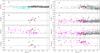 |
Fig. 3 Heavy elemental abundance ratios [X/Fe] as a function of [Fe/H]. The symbols and colours have the same meaning as in Fig. 2. Dashed lines indicate solar values. |
3.3. Elemental abundances
Abundances of α-elements (Mg, Si, Ca, Ti), iron peak elements (Cr, Ni, Zn), odd-Z elements (Na, Al), s-process elements (Sr, Y, Zr, Ba, La), r-process (Eu), and scandium were measured by fitting the selected absorption lines for each element simultaneously. Except for Ba, La, and Eu, we combined the line lists from the Bensby et al. (2003) and the Gaia-ESO line list (Heiter et al., in prep.) as we did in L15. In this work, the average abundance of Ti and Cr were derived by measuring both neutral and singly ionized lines. Since hyperfine splitting (HFS) has the effect of desaturating strong lines (McWilliam et al. 1995), we analysed the four Ba II lines by adopting the HFS from McWilliam (1998). For the La and Eu lines, we adopted the data from Lawler et al. (2001a,b), respectively. In addition, isotopes further contribute to the broadening of Ba, La, and Eu lines (e.g., Lawler et al. 2001b; Sneden et al. 2002). We assumed solar system isotopic ratios for these elements.
During the abundance analysis, we left the corresponding elemental abundance (e.g., [Na/H]) free while the stellar parameters were kept fixed. The average ratio ANa (the absolute abundance relative to the total number density of atoms) is the output from SME. The solar elemental abundance values taken from Grevesse et al. (2007) were used to normalize the SME results to obtain the abundance ratio for instance of [Na/H]. The abundance ratios with respect to Fe (i.e. [X/Fe] in standard notation) were also calculated and are shown in Figs. 2 and 3 and in Table 3. To normalize the determined abundances of our sample, we also derived solar abundances, using the same line list, and the stellar parameters derived from our solar spectrum in Sect. 3.1.
Elemental abundances of KFR08 stream members.
SME gives a typical error in abundance lower than 0.01 dex due to continuum placement and line blending. However, the uncertainties in our derived abundances are dominated by the uncertainty in stellar parameters. In Sect. 3.1 the uncertainties in the stellar parameters were found to be σTeff = 40 K, σlog g = 0.06 dex, and σ[ Fe / H ] = 0.03 dex. We calculated the uncertainties in the elemental abundances associated with these for HIP 18235 and HIP 64920. The total uncertainty, shown in Table 4, was derived by taking the square root of the quadratic sum of the different errors, as suggested by L15. The average values of the total uncertainties for all elements are between 0.03 and 0.05 dex. Although more than two lines for the r- and s-process elements were carefully selected from the literature, in some cases only a single line was used to derive the elemental abundance for a given star. This could introduce more uncertainty to the abundance than expected.
Total random errors in the abundances due to the uncertainties in stellar parameters.
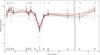 |
Fig. 4 Relative elemental abundance ratios with respect to the Sun ([X/Fe]) for all stars as a function of atomic number. When the element is Fe, the relative elemental abundance is [Fe/H]. The red dots with red lines represent the abundance patterns of the three stars tagged as cluster stars according to our chemical tagging technique (see Sect. 4), while circles with dotted lines represent the abundance patters of the other stars in our sample. The dashed line indicates the solar abundance. The grey break in the x-axis is due to the cut of blank space between Y and Ba elements. |
4. Chemical tagging
The chemical tagging method described by Mitschang et al. (2013) was employed to find out whether the KFR08 stream originates from a dissolved stellar cluster. Here we briefly summarize this method. A metric (δC) was defined as  (1)where NC is the number of measured abundances,
  and
and  are individual abundance ratios of element C with respect to Fe relative to solar for stars i and j, respectively. When the element C is Fe, then AC is the ratio of Fe to H. Here, ωC is the weighting factor for an individual species. For our purposes, this was set to unity because we do not know if any of the elements are more or less important. Furthermore, δC is the mean absolute difference between any two stars across all measured elements. To turn this δC into a probability that shows how likely it is that the stars come from a dissolved cluster, we used the empirecal probability function from Mitschang et al. (2013) that translates the δC into a probability PδC.
Given a confidence limit Plim, we first removed all pairs for which the probability is lower than this threshold. Secondly, all the remaining candidates that make up the pairs were re-evaluated based on their δC and PδC. In this way, we separated the potential dissolved clusters stars from the field stars using their elemental abundances. As Mitschang et al. (2013) suggested, the cluster detection confidence, Pclus, was finally evaluated using the mean of δC in the tagged group.
Two confidence limits of 85% and 68% were used to verify whether the stream comes from a dissolved cluster or not. The 68% threshold, which is analogous to a 1σ detection, is the lowest meaningful probability and corresponds to a δC of 0.058 dex, which is comparable with the systematic uncertainty in the abundances. As Mitschang et al. (2013) pointed out, a linked group of stars is less contaminated by other groups if a higher confidence level is used (Plim = 85%).
We were unable to obtain abundances of [Sr/Fe], [Zr/Fe] and [La/Fe] for three stars because the absorption lines are weak. Thus we used the abundances of 14 elements (Na, Mg, Al, Si, Ca, Sc, Ti, Cr, Fe, Ni, Zn, Y, Ba, and Eu) to identify the stream members. We found that three stars, HIP 18235, HIP 58843, and HIP 74033, could belong to one group using a limit of Plim = 68%. The mean δC of the three stars is 0.044, which gives a group detection confidence of ~84%. No star was tagged as a member of a group of stars when we tested with a higher threshold (Plim = 85%).
In Fig. 4, we show the abundance patterns of the three tagged cluster stars in comparison with the other stream stars. The figure shows that the three stars (shown as red filled diamonds) have almost the same elemental abundances within the uncertainties. If all stars originated from a single star cluster, we would expect that they exhibit similar abundance ratios in all elements. This can be seen for some elements, such as Mg, Cr, and Ni. The scatter of abundance ratios among our sample stars for those elements are between 0.04 and 0.08 dex, which is comparable with or somewhat higher than, the measurement uncertainty. However, the stars have very a large scatter (σ[ X / Fe ] ≥ 0.12 dex) in abundance ratios in other elements, such as Na, Al, Ti, Y, Ba, and Eu. The metallicity, [Fe/H], exhibited the largest dispersion with σ[ Fe / H ] = 0.29. These large dispersions suggest that the stars have different birthplaces. As shown in Fig. 4, the star-to-star scatter of chemical composition of the three tagged stars is significantly different from that of other stars. This illustrates that our chemical tagging method, based on the selection of 14 elements, is efficient in isolating the cluster stars from the field stars.
As mentioned before, the stellar parameters based on the parallaxes were computed using Procedure 2 for our sample. Then, we measured their elemental abundances using derived stellar parameters in the same way as introduced in Sect. 3. The same three stars were identified as cluster members when we followed the same chemical tagging experiment as before.
5. Discussion
5.1. Is the KFR08 stream a dissolved cluster?
Recent studies of observations (see De Silva et al. 2007a; Pancino et al. 2010) and simulations (Feng & Krumholz 2014) demonstrated that chemical compositions within stellar clusters are homogenous. The stream stars should have the same elemental abundances and stellar age if the KFR08 stream originated from a cluster. As mentioned in Sect. 4, the star-to-star scatter in abundances of most elements is quite large compared to the measurement uncertainty. The sample stars spread in abundances space rather than cluster together. We also found that 4 of the 16 stars (see Table 2) are much younger than the other members. This suggests that at least a fraction of the stream members are not from a dissolved cluster.
How likely is it that the three stars we found to belong to a chemically homogenous cluster in Sect. 4 really come from a dissolved cluster and are not a chance grouping? Mitschang et al. (2013) predicted that half of the members in a chemically tagged group in fact are interlopers when a confidence limit of 68% is used. Thus, it is possible that the three stars found in Sect. 4 do not belong to a chemically homogenous group of stars, or in other words, a dissolved cluster. This is supported by our higher confidence level experiment that no star is linked to a group when the threshold is set to 85%.
In addition, if we assumed that the three stars HIP 18235, HIP 58843, and HIP 74033 are siblings of a dissolved cluster, they should have similar RVs. However, we found that the difference in their RVs is larger than 50 km s-1 (see Table 2). We also might expect the three stars to have similar kinematics if they were born in the cluster. When we examined their angular momenta (see Fig. 5) and total velocities (see Fig. 6), however, they are not more clustered than other stars in the angular momentum and velocity spaces. This further weakens the likelihood that they are part of a dissolved stellar cluster.
The probability that the star HIP 74033 belongs to the KFR08 stream is 0.65 according to Bobylev et al. (2010). Since the location of this star in velocity space is also close to the Arcturus stream, we are not surprised that it was selected as a potential member of the Arcturus stream in Arifyanto & Fuchs (2006). Thus the nature of this star and which stream it might belong to is rather unclear.
Although we found that three stream candidates have similar elemental abundances, from this discussion we conclude that they do not belong to a dissolved cluster.
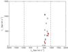 |
Fig. 5 Distribution of the stream candidates in angular momentum (Lz and L⊥)-space. We note that the distance of the local standard of rest to the Galactic centre is R⊙ = 8.5 kpc. The coloured diamonds have the same meaning as in Fig. 2. Two dashed lines are used to illustrate the angular momenta to typical halo stars. |
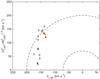 |
Fig. 6 Toomre diagram. The two circles delineate constant total space velocities of vtot = 70 and 200 km s-1, respectively. The coloured diamonds have the same meaning as in Fig. 2. |
5.2. Does the KFR08 originate from an accreted galaxy?
A possible origin for the KFR08 stream is that it is part of the tidal debris from a satellite accreted long ago. Such a minor merger origin was proposed by Klement et al. (2008). A significant population of stars, which lag behind the LSR by ~100 km s-1, with kinematics intermediate between the canonical thick disc and the stellar halo were interpreted as remnants of a merger by Gilmore et al. (2002) and Wyse et al. (2006). Gilmore et al. (2002) also found more evidence that the stellar halo retains kinematic substructure that is indicative of minor mergers. Our sample has V velocity ≃ −152 km s-1 with respect to the LSR. The stream candidates selected by Klement et al. (2008) from the RAVE survey look like halo stars and show quite radial orbits (high W velocities). The mean W velocity of our sample is  . We calculated the angular momenta of our stream members. These are shown in Fig. 5. We found that the stars cluster around Lz = 500 kpc km s-1. This suggests that they might belong to the halo population. We also found that the stars have large scatter in the
  component. Thus, they do not show any difference when we compare them with the distribution of normal halo stars in Lz and L⊥ space (e.g., Kepley et al. 2007).
Chemically, our stars have [α/Fe] ratios that are enhanced for any given α-element. This is distinct from the low ratios observed in surviving dwarf satellite galaxies (e.g., Tolstoy et al. 2009, also see Sect. 5.3). Thus, if the KFR08 stars were accreted, they must have come from a merger with a more massive satellite galaxy. In this case, the stars could have lower W velocities, as in our observations, since they would be dragged into the plane of the Milky Way by dynamical frication (e.g., Read et al. 2008; Ruchti et al. 2014).
In addition to the dynamical arguments given above, Venn et al. (2004) demonstrated that the thick disc cannot be comprised of the remnants from a low-mass dwarf spheroidal (dSph) galaxy because dSph galaxies are α-poor when compared to the Galactic stars of similar [Fe/H]. As can be seen in Figs. 2 and 3, the stream candidates are α enhanced and [Fe/H] of the stars cover a broad range.
5.3. Does the KFR08 stream have a dynamical origin?
For the s-and r-process elements, such as Ba, La, and Eu, a large scatter in abundance ratios is seen in Fig. 3. Since they are produced in different places and on differnt timescales, this implies that our candidates might have different birth places. We collected a large sample consisting of thin and thick-disc and halo stars from the literature (Fulbright 2000; Nissen & Schuster 2010; Bensby et al. 2014) and show these stars together with our data in Figs. 2 and 3. As can be seen, the abundance patterns of our sample stars matched the thick-disc population well. It has been shown that the Eu abundance follows the Mg abundance in thin- and thick-disc stars, while halo stars show an overabundance of Eu relative to Mg (Mashonkina & Gehren 2001; Mashonkina et al. 2003). For our sample stars, the mean value [ Eu / Mg ] = −0.02 ± 0.20 is consistent with the trends found for the thick-disc stars.
Generally, stars with a total velocity vtot ≡ (U2 + V2 + W2)1 / 2 greater than ~70 km s-1, but less than ~200 km s-1, are likely to be thick-disc stars (e.g., Nissen 2004). According to data presented in the Toomre diagram (Fig. 6), the kinematics of the KFR08 stream is intermediate between the thick disc and halo populations. Combining with the chemical signature of thick disc for the stream stars, they might have once belonged to the thick disc and gained hot kinematics as a result of a satellite merger. This is consistent with the hypothesis suggested by Minchev et al. (2009) that the high-velocity KFR08 stream has a dynamical origin presumably due to a strong perturbation in the Galactic disc from a merger.
As mentioned before, our sample stars have a large dispersion in W velocity. The U velocities also have a large scatter with σU ~ 86 km s-1. We have shown that the KFR08 stream is older than 11 Gyr. Such an old populations with a high-velocity dispersion could be expected if they were perturbed by massive mergers in the early Universe (Minchev et al. 2014). It is also possible that the stars subsequently migrated from the inner disc to their current position. However, it is unclear how much radial migration would increase the velocity dispersion of the stars (Minchev et al. 2013; Vera-Ciro et al. 2014).
6. Conclusions
We derived the stellar parameters and elemental abundances for 16 of the KFR08 stream members identified by Bobylev et al. (2010) by comparing synthetic with observed spectra. The stellar ages were also obtained by fitting to isochrones. To determine whether the stream is a dissolved cluster, a chemical tagging method was used to tag the cluster members. We found that three stars have similar abundances and could belong to one group using a confidence limit of Plim = 68%. However, further tests (see Sect. 5.1) do not support the conclusion that the three chemically similar stars come from a dissolved cluster.
As an alternative to a dissolved cluster origin, the stream could originate from an accreted satellite galaxy or have a dynamical origin caused by a massive merger. Klement et al. (2008) proposed that the KFR08 stream is part of the tidal debris from a satellite accreted long ago. Although the stream stars cluster around angular momentum Lz = 500 kpc km s-1, they have a large scatter in the L⊥ component. This makes them similar to the field halo stars in Lz and L⊥ space. The mean U and W velocities of our sample are very low with respect to the LSR. This might be inconsistent with the hypothesis that the KFR08 stream was accreted from a dwarf satellite galaxy.
We furthermore found that the stream members are α-enhanced. This strongly speaks against the accretion debris origin of stream if we expect the KFR08 stream progenitor to be similar to present-day dSph galaxies. It has been noted that a high-mass dwarf galaxy has a higher rate of star formation than the remaining satellite of the Milky Way, and their metallicity can be enriched to [Fe/H] = –0.6 (Tamura et al. 2001). We therefore cannot rule out a satellite progenitor of the stream, which has a substantial mass similar to the LMC or Sgr dwarf galaxy. We found that the abundance patterns of stream stars matched the thick-disc population well, especially for the [Eu/Mg]. In addition to the very old ages (>11 Gyr), the stream stars have hotter kinematics than the canonical thick-disc stars. A more likely scenario is thus that the members of the KFR08 stream have a dynamical origin due to a strong perturbation from a merger event in the early Universe.
Acknowledgments
The authors would like to thank Thomas Bensby for valuable stellar ages that improved the analysis of the paper. This project was completed under the GREAT – ITN network, which is funded through the European Union Seventh Framework Programme [FP7/2007-2013] under grant agreement No. 264895. S.F. is funded by grant No. 621-2011-5042 from The Swedish Research Council. G.R. is funded by the project grant “The New Milky Way” from the Knut and Alice Wallenberg Foundation. This research made use of the SIMBAD database, operated at the CDS, Strasbourg, France.
References
- Abazajian, K. N., Adelman-McCarthy, J. K., Agüeros, M. A., et al. 2009, ApJS, 182, 543 [NASA ADS] [CrossRef] [Google Scholar]
- Alonso, A., Arribas, S., & Martinez-Roger, C. 1996, A&A, 313, 873 [NASA ADS] [Google Scholar]
- Antoja, T., Valenzuela, O., Pichardo, B., et al. 2009, ApJ, 700, L78 [NASA ADS] [CrossRef] [Google Scholar]
- Arifyanto, M. I., & Fuchs, B. 2006, A&A, 449, 533 [NASA ADS] [CrossRef] [EDP Sciences] [Google Scholar]
- Bensby, T., Feltzing, S., & Lundström, I. 2003, A&A, 410, 527 [NASA ADS] [CrossRef] [EDP Sciences] [Google Scholar]
- Bensby, T., Oey, M. S., Feltzing, S., & Gustafsson, B. 2007, ApJ, 655, L89 [NASA ADS] [CrossRef] [Google Scholar]
- Bensby, T., Adén, D., Meléndez, J., et al. 2011, A&A, 533, A134 [NASA ADS] [CrossRef] [EDP Sciences] [Google Scholar]
- Bensby, T., Feltzing, S., & Oey, M. S. 2014, A&A, 562, A71 [NASA ADS] [CrossRef] [EDP Sciences] [Google Scholar]
- Bergemann, M., Lind, K., Collet, R., Magic, Z., & Asplund, M. 2012, MNRAS, 427, 27 [NASA ADS] [CrossRef] [Google Scholar]
- Bland-Hawthorn, J., Krumholz, M. R., & Freeman, K. 2010, ApJ, 713, 166 [NASA ADS] [CrossRef] [Google Scholar]
- Bobylev, V. V., Bajkova, A. T., & Mylläri, A. A. 2010, Astron. Lett., 36, 27 [NASA ADS] [CrossRef] [Google Scholar]
- De Silva, G. M., Freeman, K. C., Asplund, M., et al. 2007a, AJ, 133, 1161 [NASA ADS] [CrossRef] [Google Scholar]
- De Silva, G. M., Freeman, K. C., Bland-Hawthorn, J., Asplund, M., & Bessell, M. S. 2007b, AJ, 133, 694 [NASA ADS] [CrossRef] [Google Scholar]
- Dehnen, W. 1998, AJ, 115, 2384 [NASA ADS] [CrossRef] [Google Scholar]
- Dehnen, W. 2000, AJ, 119, 800 [NASA ADS] [CrossRef] [Google Scholar]
- Dekker, H., D’Odorico, S., Kaufer, A., Delabre, B., & Kotzlowski, H. 2000, in Optical and IR Telescope Instrumentation and Detectors, eds. M. Iye, & A. F. Moorwood, SPIE Conf. Ser., 4008, 534 [Google Scholar]
- Demarque, P., Woo, J.-H., Kim, Y.-C., & Yi, S. K. 2004, ApJS, 155, 667 [NASA ADS] [CrossRef] [Google Scholar]
- Eggen, O. J. 1978, ApJ, 222, 191 [NASA ADS] [CrossRef] [Google Scholar]
- Famaey, B., Jorissen, A., Luri, X., et al. 2005, A&A, 430, 165 [NASA ADS] [CrossRef] [EDP Sciences] [Google Scholar]
- Feltzing, S., & Holmberg, J. 2000, A&A, 357, 153 [NASA ADS] [Google Scholar]
- Feng, Y., & Krumholz, M. R. 2014, Nature, 513, 523 [NASA ADS] [CrossRef] [Google Scholar]
- Fulbright, J. P. 2000, AJ, 120, 1841 [NASA ADS] [CrossRef] [Google Scholar]
- Gilmore, G., Wyse, R. F. G., & Norris, J. E. 2002, ApJ, 574, L39 [NASA ADS] [CrossRef] [Google Scholar]
- Grevesse, N., Asplund, M., & Sauval, A. J. 2007, Space Sci. Rev., 130, 105 [Google Scholar]
- Gustafsson, B., Edvardsson, B., Eriksson, K., et al. 2008, A&A, 486, 951 [NASA ADS] [CrossRef] [EDP Sciences] [Google Scholar]
- Helmi, A., White, S. D. M., de Zeeuw, P. T., & Zhao, H. 1999, Nature, 402, 53 [NASA ADS] [CrossRef] [Google Scholar]
- Helmi, A., Navarro, J. F., Meza, A., Steinmetz, M., & Eke, V. R. 2003, ApJ, 592, L25 [NASA ADS] [CrossRef] [Google Scholar]
- Helmi, A., Navarro, J. F., Nordström, B., et al. 2006, MNRAS, 365, 1309 [NASA ADS] [CrossRef] [Google Scholar]
- Holmberg, J., Nordström, B., & Andersen, J. 2007, A&A, 475, 519 [NASA ADS] [CrossRef] [EDP Sciences] [MathSciNet] [Google Scholar]
- Ibata, R. A., Gilmore, G., & Irwin, M. J. 1994, Nature, 370, 194 [NASA ADS] [CrossRef] [Google Scholar]
- Kaufer, A., Stahl, O., Tubbesing, S., et al. 1999, The Messenger, 95, 8 [Google Scholar]
- Kepley, A. A., Morrison, H. L., Helmi, A., et al. 2007, AJ, 134, 1579 [NASA ADS] [CrossRef] [Google Scholar]
- Klement, R., Fuchs, B., & Rix, H.-W. 2008, ApJ, 685, 261 [NASA ADS] [CrossRef] [Google Scholar]
- Klement, R., Rix, H.-W., Flynn, C., et al. 2009, ApJ, 698, 865 [NASA ADS] [CrossRef] [Google Scholar]
- Klement, R. J., Bailer-Jones, C. A. L., Fuchs, B., Rix, H.-W., & Smith, K. W. 2011, ApJ, 726, 103 [NASA ADS] [CrossRef] [Google Scholar]
- Lawler, J. E., Bonvallet, G., & Sneden, C. 2001a, ApJ, 556, 452 [NASA ADS] [CrossRef] [Google Scholar]
- Lawler, J. E., Wickliffe, M. E., den Hartog, E. A., & Sneden, C. 2001b, ApJ, 563, 1075 [CrossRef] [Google Scholar]
- Liu, C., Ruchti, G., Feltzing, S., et al. 2015, A&A, 575, A51 [NASA ADS] [CrossRef] [EDP Sciences] [Google Scholar]
- Mashonkina, L., & Gehren, T. 2001, A&A, 376, 232 [NASA ADS] [CrossRef] [EDP Sciences] [Google Scholar]
- Mashonkina, L., Gehren, T., Travaglio, C., & Borkova, T. 2003, A&A, 397, 275 [NASA ADS] [CrossRef] [EDP Sciences] [Google Scholar]
- Mayor, M., Pepe, F., Queloz, D., et al. 2003, The Messenger, 114, 20 [NASA ADS] [Google Scholar]
- McWilliam, A. 1998, AJ, 115, 1640 [NASA ADS] [CrossRef] [Google Scholar]
- McWilliam, A., Preston, G. W., Sneden, C., & Searle, L. 1995, AJ, 109, 2757 [NASA ADS] [CrossRef] [Google Scholar]
- Minchev, I., Quillen, A. C., Williams, M., et al. 2009, MNRAS, 396, L56 [NASA ADS] [CrossRef] [Google Scholar]
- Minchev, I., Chiappini, C., & Martig, M. 2013, A&A, 558, A9 [NASA ADS] [CrossRef] [EDP Sciences] [Google Scholar]
- Minchev, I., Chiappini, C., Martig, M., et al. 2014, ApJ, 781, L20 [NASA ADS] [CrossRef] [Google Scholar]
- Mitschang, A. W., De Silva, G., Sharma, S., & Zucker, D. B. 2013, MNRAS, 428, 2321 [NASA ADS] [CrossRef] [Google Scholar]
- Navarro, J. F., Helmi, A., & Freeman, K. C. 2004, ApJ, 601, L43 [NASA ADS] [CrossRef] [Google Scholar]
- Nissen, P. E. 2004, in Origin and Evolution of the Elements, eds. A. McWilliam, & M. Rauch (Pasadena: Carnegie Observatories) 154 [Google Scholar]
- Nissen, P. E., & Schuster, W. J. 2010, A&A, 511, L10 [NASA ADS] [CrossRef] [EDP Sciences] [Google Scholar]
- Nordström, B., Mayor, M., Andersen, J., et al. 2004, A&A, 418, 989 [NASA ADS] [CrossRef] [EDP Sciences] [Google Scholar]
- Olsen, E. H. 1983, A&AS, 54, 55 [NASA ADS] [Google Scholar]
- Olsen, E. H. 1993, A&AS, 102, 89 [NASA ADS] [Google Scholar]
- Pancino, E., Carrera, R., Rossetti, E., & Gallart, C. 2010, A&A, 511, A56 [NASA ADS] [CrossRef] [EDP Sciences] [Google Scholar]
- Perryman, M. A. C., Lindegren, L., Kovalevsky, J., et al. 1997, A&A, 323, L49 [NASA ADS] [Google Scholar]
- Read, J. I., Lake, G., Agertz, O., & Debattista, V. P. 2008, MNRAS, 389, 1041 [NASA ADS] [CrossRef] [Google Scholar]
- Ruchti, G. R., Bergemann, M., Serenelli, A., Casagrande, L., & Lind, K. 2013, MNRAS, 429, 126 [NASA ADS] [CrossRef] [Google Scholar]
- Ruchti, G. R., Read, J. I., Feltzing, S., Pipino, A., & Bensby, T. 2014, MNRAS, 444, 515 [Google Scholar]
- Schuster, W. J., & Nissen, P. E. 1988, A&AS, 73, 225 [NASA ADS] [Google Scholar]
- Sneden, C., Cowan, J. J., Lawler, J. E., et al. 2002, ApJ, 566, L25 [Google Scholar]
- Steinmetz, M., Zwitter, T., Siebert, A., et al. 2006, AJ, 132, 1645 [NASA ADS] [CrossRef] [Google Scholar]
- Tamura, N., Hirashita, H., & Takeuchi, T. T. 2001, ApJ, 552, L113 [NASA ADS] [CrossRef] [Google Scholar]
- Tolstoy, E., Hill, V., & Tosi, M. 2009, ARA&A, 47, 371 [NASA ADS] [CrossRef] [Google Scholar]
- Torres, G. 2010, AJ, 140, 1158 [NASA ADS] [CrossRef] [Google Scholar]
- Valenti, J. A., & Fischer, D. A. 2005, ApJS, 159, 141 [NASA ADS] [CrossRef] [MathSciNet] [Google Scholar]
- Valenti, J. A., & Piskunov, N. 1996, A&AS, 118, 595 [NASA ADS] [CrossRef] [EDP Sciences] [Google Scholar]
- van Leeuwen, F. 2007, A&A, 474, 653 [NASA ADS] [CrossRef] [EDP Sciences] [Google Scholar]
- Venn, K. A., Irwin, M., Shetrone, M. D., et al. 2004, AJ, 128, 1177 [NASA ADS] [CrossRef] [Google Scholar]
- Vera-Ciro, C., D’Onghia, E., Navarro, J., & Abadi, M. 2014, ApJ, 794, 173 [NASA ADS] [CrossRef] [Google Scholar]
- Wyse, R. F. G., Gilmore, G., Norris, J. E., et al. 2006, ApJ, 639, L13 [NASA ADS] [CrossRef] [Google Scholar]
All Tables
Galactic coordinates, distances, space velocities, radial velocities, masses, absolute magnitudes, and ages of KFR08 stream members.
Total random errors in the abundances due to the uncertainties in stellar parameters.
All Figures
|
Fig. 1 Teff vs. log g diagram. Filled circles indicate our main sample from the Hipparcos catalogue. Isochrones at different ages (10 and 13 Gyr) and metallicities (–0.6 and –1.0 dex) according to the Yonsei-Yale models (Demarque et al. 2004) are shown. |
| In the text | |
|
Fig. 2 Light elemental abundance ratios [X/Fe] as a function of [Fe/H]. Three tagged cluster stars (see Sect. 4) are indicated as red filled diamonds, while other stream stars are shown as black emptied diamonds. The disc stars from Bensby et al. (2014) are plotted as open gray circles, while the cyan triangles and magenta stars indicate the thick-disc and halo stars collected from Nissen & Schuster (2010) and Fulbright (2000), respectively. Dashed lines indicate solar values. |
| In the text | |
|
Fig. 3 Heavy elemental abundance ratios [X/Fe] as a function of [Fe/H]. The symbols and colours have the same meaning as in Fig. 2. Dashed lines indicate solar values. |
| In the text | |
|
Fig. 4 Relative elemental abundance ratios with respect to the Sun ([X/Fe]) for all stars as a function of atomic number. When the element is Fe, the relative elemental abundance is [Fe/H]. The red dots with red lines represent the abundance patterns of the three stars tagged as cluster stars according to our chemical tagging technique (see Sect. 4), while circles with dotted lines represent the abundance patters of the other stars in our sample. The dashed line indicates the solar abundance. The grey break in the x-axis is due to the cut of blank space between Y and Ba elements. |
| In the text | |
|
Fig. 5 Distribution of the stream candidates in angular momentum (Lz and L⊥)-space. We note that the distance of the local standard of rest to the Galactic centre is R⊙ = 8.5 kpc. The coloured diamonds have the same meaning as in Fig. 2. Two dashed lines are used to illustrate the angular momenta to typical halo stars. |
| In the text | |
|
Fig. 6 Toomre diagram. The two circles delineate constant total space velocities of vtot = 70 and 200 km s-1, respectively. The coloured diamonds have the same meaning as in Fig. 2. |
| In the text | |
Current usage metrics show cumulative count of Article Views (full-text article views including HTML views, PDF and ePub downloads, according to the available data) and Abstracts Views on Vision4Press platform.
Data correspond to usage on the plateform after 2015. The current usage metrics is available 48-96 hours after online publication and is updated daily on week days.
Initial download of the metrics may take a while.