| Issue |
A&A
Volume 579, July 2015
|
|
|---|---|---|
| Article Number | A14 | |
| Number of page(s) | 10 | |
| Section | Planets and planetary systems | |
| DOI | https://doi.org/10.1051/0004-6361/201526138 | |
| Published online | 19 June 2015 | |
Inner main belt asteroids in Slivan states?
Institute of Astronomy, Charles University, V Holešovičkách 2, 180 00 Prague 8, Czech Republic
e-mail: This email address is being protected from spambots. You need JavaScript enabled to view it.
, This email address is being protected from spambots. You need JavaScript enabled to view it.
Received: 19 March 2015
Accepted: 27 April 2015
Abstract
Context. The spin state of ten asteroids in the Koronis family has previously been determined. Surprisingly, all four asteroids with prograde rotation were shown to have spin axes nearly parallel in the inertial space. All asteroids with retrograde rotation had large obliquities and rotation periods that were either short or long. The Yarkovsky-O’Keefe-Radzievskii-Paddack (YORP) effect has been demonstrated to be able to explain all these peculiar facts. In particular, the effect causes the spin axes of the prograde rotators to be captured in a secular spin-orbit resonance known as Cassini state 2, a configuration dubbed “Slivan state”.
Aims. It has been proposed based on an analysis of a sample of asteroids in the Flora family that Slivan states might also exist in this region of the main belt. This is surprising because convergence of the proper frequency s and the planetary frequency s6 was assumed to prevent Slivan states in this zone. We therefore investigated the possibility of a long-term stable capture in the Slivan state in the inner part of the main belt and among the asteroids previously observed.
Methods. We used the swift integrator to determine the orbital evolution of selected asteroids in the inner part of the main belt. We also implemented our own secular spin propagator into the swift code to efficiently analyze their spin evolution.
Results. Our experiments show that the previously suggested Slivan states of the Flora-region asteroids are marginally stable for only a small range of the flattening parameter Δ. Either the observed spins are close to the Slivan state by chance, or additional dynamical effects that were so far not taken into account change their evolution. We find that only the asteroids with very low-inclination orbits (lower than ≃4°, for instance) could follow a similar evolution path as the Koronis members and be captured in their spin state into the Slivan state. A greater number of asteroids in the inner main-belt Massalia family, which are at a slightly larger heliocentric distance and at lower inclination orbits than in the Flora region, may have their spin in the Slivan state.
Key words: celestial mechanics / minor planets, asteroids: general
© ESO, 2015
1. Introduction
The past decade has seen an enormous increase in the number of asteroids for which astronomical observations allowed resolving the rotation pole orientation in space (e.g., Ďurech et al. 2015, and references therein). This wealth of data allows new studies of asteroids and their populations. One of the early examples of such results was a discovery of Slivan states among the Koronis family members (Slivan 2002; Slivan et al. 2009). The most striking element in this dataset consisted of a group of prograde-rotating asteroids with spin axes nearly parallel in inertial space and similar rotation periods (later dubbed the Slivan states). A model that explains this situation, proposed by Vokrouhlický et al. (2003), is based on the idea that the spin axis is confined in resonance between its precession rate by solar torques and a particular mode of these asteroids’ orbit precession in the inertial space. Because the latter is common to all bodies in the main belt and because it derives from the current configuration of giant planets, it explains the preferred direction in the inertial space. Additionally, Vokrouhlický et al. (2003) proved that this resonant state is an attractor of a long-term evolution driven by the Yarkovsky-O’Keefe-Radzievskii-Paddack (YORP) torques. Hence, despite their tiny volume in phase and parametric spaces, one may expect asteroids with spin states to populate this resonance with a reasonable probability. Because the notion of this resonant state is central to this paper as well, we briefly recall its dynamical principle in Sect. 2.11.
Vokrouhlický et al. (2003) also mentioned that conditions favorable for existence of the Slivan states occur in the outer parts of the main belt and for asteroids on low-inclination orbits. On the other hand, their appearance in the inner part of the main belt (heliocentric distance smaller than 2.5 au) seemed problematic. Results in the recent study of the Flora-region asteroids by Kryszczyńska, summarized by two papers Kryszczyńska et al. (2012) and Kryszczyńska (2013), thus appear as a surprise2. In particular, Kryszczyńska (2013) determined the spin vector orientation of nearly 20 asteroids and found that many of the prograde-rotating bodies possibly appear to be locked in Slivan states. This situation motivates us to examine the conditions of existence of Slivan states in the inner main belt, and in particular among the asteroids observed by Kryszczyńska (2013).
2. Methods
2.1. Brief review of the theory
We consider a main-belt asteroid that rotates about the shortest axis of the inertia tensor. We denote its angular velocity of rotation by ω and the direction of the spin axis by a unit vector s. We assume that the solar gravitational field produces the only torque relevant for the spin state evolution and we are not interested in variations of ω and s with periods similar to or shorter than its revolution about the Sun. This easily leads to (i) ω is constant; and (ii) the spin axis direction s evolves in any inertial frame according to (e.g., Colombo 1966; Bertotti et al. 2003)  (1)Here c denotes a unit vector in the direction of the asteroid’s orbital angular momentum and
  (2)where
  , e is the orbital eccentricity, n is the orbital mean motion, and Δ depends on the asteroid’s principal moments of inertia (A,B,C)
 (3)(we assume A ≤ B ≤ C).
If the orbital plane were fixed in the inertial space, Eq. (1) would have a simple solution, namely a steady precession of s about c at a constant angular distance ε (cosε = s·c) and with a frequency αcosε. The situation becomes more complicated and interesting when the time evolution of c is taken into account. This is relevant because the asteroid’s orbital plane evolves due to planetary perturbations on a timescale similar to the period of precession estimated from this simple model.
It has been argued that the dynamics of s is more conveniently described in a reference frame that co-moves with the orbital plane in which simply cT = (0,0,1). Because this new system is not inertial, the simplicity of the description of c is paid for by the occurrence of new (non-inertial) torques on the right-hand side of Eq. (1). In particular, by denoting with A the transformation matrix between the inertial frame ℰ, which is suitable to describe the asteroid’s orbital evolution, and the co-moving frame ℰ′, one obtains the following expression for the additional torques:  (4)Because the matrix (dA/dt) AT is skew symmetric, its three off-diagonal terms may be organized into a vector quantity h, such that Tin = −h × s. As a result, the dynamical equations for the spin axis evolution now take the following form:
 ![Mathematical equation: \begin{eqnarray} \frac{{\rm d}{\vec s}}{{\rm d}t} = -\left[\alpha \left({\vec c}\cdot{\vec s}\right) {\vec c}+{\vec h}\right] \times {\vec s}. \label{sdyn3} \end{eqnarray}](/articles/aa/full_html/2015/07/aa26138-15/aa26138-15-eq28.png) (5)The orientation of the orbital plane in ℰ, set by c, is parametrically described by the orbital longitude of node Ω and inclination I. Indefiniteness of the nodal line, and the associated singularity in the dynamical equations, when I becomes very small, may be conveniently eliminated by a suitable choice of the reference direction in the ℰ′. To do this, the transformation between ℰ and ℰ′ is chosen using a 3-1-3 sequence of the Euler angles (Ω,I,−Ω), and thus A = R3(−Ω)R1(I)R3(Ω). Here, R1 and R3 are rotational matrixes about the x and z directions of a given reference frame. In this case,
(5)The orientation of the orbital plane in ℰ, set by c, is parametrically described by the orbital longitude of node Ω and inclination I. Indefiniteness of the nodal line, and the associated singularity in the dynamical equations, when I becomes very small, may be conveniently eliminated by a suitable choice of the reference direction in the ℰ′. To do this, the transformation between ℰ and ℰ′ is chosen using a 3-1-3 sequence of the Euler angles (Ω,I,−Ω), and thus A = R3(−Ω)R1(I)R3(Ω). Here, R1 and R3 are rotational matrixes about the x and z directions of a given reference frame. In this case,  with
with 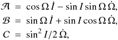 (6)where overdots mean time derivatives.
While not necessarily convenient for numerical integration, the spin vector s may be parametrized with two angular parameters. By long tradition in astronomy, they have most often been chosen such that  (7)where ε is the obliquity and ψ the precession angle. The two independent dynamical equations for ε and ψ take a form of Hamilton equations associated with a Hamiltonian (e.g., Ward 1975; Henrard & Murigande 1987; Laskar & Robutel 1993; Neron de Surgy & Laskar 1997; Vokrouhlický et al. 2006c),
  (8)where (X = cosε,ψ) are canonical variables, X is the momentum and ψ the conjugated coordinate. Even though ℋ is one-dimensional, a solution in form of a quadrature cannot be found. This is because coefficients
  , and in principle also α via the eccentricity evolution, explicitly depend on time and the problem does not admit an energy integral. Definitions (6) may be more conveniently rewritten using a complex, and nonsingular, quantity ζ = sin(I/ 2) exp(ıΩ), namely
  where
where  is the complex unit and
  is complex conjugate to ζ. For a small enough orbital inclination I, Eqs. (9) and (10) reveal that to a linear approximation in I (i)
  ; and (ii)
  . The linear analytical theory of the asteroid secular evolution provides insights into the time dependence of ζ, namely its representation by a finite number of harmonic terms ζ = ∑ Aiexp [ı(νit + φi)]. Nonlinear corrections, and/or an analysis of numerically integrated orbital evolution, typically add more terms in this Fourier representation, but do not modify its principal character.
Vokrouhlický et al. (2006c) showed that for (i) high-inclination orbits, such as in the Phocaea region, the harmonic representation of ζ is dominated by a single (proper) term; while at (ii) lower inclinations typically two contributions compete, the proper term and a forced term associated with the s6 planetary frequency. The presence of other terms in the ζ harmonic development usually contributes as a weak perturbation. A toy model that assumes only a single harmonic term in ζ, easily applicable to (i) and a point of guidance in (ii), is generally known as the Colombo top problem (e.g., Colombo 1966; Henrard & Murigande 1987). While necessarily approximate, concepts introduced in the Colombo top model are crucial for understanding Slivan states, and we thus briefly recall the main results.
The single-line case, when ζ = A exp [ı(st + φ)], corresponds to the situation of a constant orbital inclination I (A = sinI/ 2) to a reference plane in ℰ, and a steady precession of the node (Ω = st + φ). At a first glance, not much is changed since the Hamiltonian (8) is still time-dependent. But a simple canonical transformation helps to remove this time dependence (assuming orbital eccentricity, and thus α, is constant). The new canonical variables (X′,ϕ) are defined by X′ = −X and3ϕ = −(ψ + Ω), and the new Hamiltonian now takes the form  (11)Since ℋ′ may obviously be scaled by any constant, it depends on only two dimensionless parameters κ = α/ (2s) and I. The time independence of the new Hamiltonian (11) enforces the first integral ℋ′ = C, which in principle may lead to an analytic solution of the problem (Breiter et al., in prep.). We focus here on the general knowledge of the phase flow from the first integral itself, however. Its makeup follows from a number of stationary solutions of the Colombo problem4. Depending on the value of κ, there might be two or four stationary solutions: (i) | κ | <κ⋆ implies two stationary solutions; and (ii) | κ | >κ⋆ implies four stationary solutions, with (e.g., Henrard & Murigande 1987)5
 (12)The stationary solutions have either ϕ = 0° or ϕ = 180°, and the obliquity value satisfies
  (13)with the upper sign − for ϕ = 0° and lower sign + for ϕ = 180°. Of particular interest is the ϕ = 0° stationary point when | κ | >κ⋆ (four stationary solutions), which is usually referred to as Cassini state 2 (C2). This is because the phase flow around C2 is characteristic of a resonant situation with ϕ librating in a limited interval of values. In fact, the stable C2 solution is associated with one of the stationary points at ϕ = 180° (Cassini state 4, C4) that is unstable, such that the isolines ℋ′ = C meeting at C4 constitute a separatrix of the flow around C2 (Fig. 1). To understand the nature of the resonance in this case, one may use Eq. (13). Assuming that the obliquity ε is higher than the orbital inclination, we have αcosε ≃ −s. We recall that the left-hand side here is the precession rate of s due to the solar gravitational torque, and thus C2 state is a 1:1 resonance between the spin axis precession and the orbital plane precession in space. The maximum resonance width Δε may be determined from (e.g., Henrard & Murigande 1987; Ward & Hamilton 2004; Vokrouhlický et al. 2006c)
  (14)where ε4 is obliquity of the unstable equilibrium from Eq. (13). Note that ε4 has a minimum, nonzero value atan(tan1/3I) when | κ | = κ⋆ and asymptotically approaches 90° for | κ | → ∞. At this limit Δε → 0, because κsin2ε4 is still finite according to Eq. (13). Equation (14) shows the dependence of the orbital inclination on the square root, so even when I is small (a few degrees, for instance), the width of the resonance zone may be large (tens of degrees, for instance). This is important for the above-mentioned case of asteroids on low-inclination orbits in the main belt, because the Fourier representation of ζ requires at least two terms (unlike in the Colombo model, where only one term is present). We may formally construct the orbital reference frame ℰ′ associated with each of the two contributing terms and apply the concepts of the Colombo top model, but the second term will always introduce a perturbation. For instance, the characteristic amplitude of the perturbation in obliquity is on the order of the orbital inclination of the orbital frame associated with the perturbing term. Motion in the resonant zone about the C2 point may, however, withstand these perturbations provided the extent of the zone is large enough.
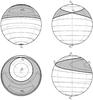 |
Fig. 1 Isolines ℋ′ = C on a unit sphere for the Colombo top model with I = 5° and κ = −0.914; since | κ | >κ⋆ ≃ 0.652 there are four stationary (Cassini) equilibria of the flow denoted by symbols and labeled C1 to C4. The resonant zone about C2 is highlighted by gray shading. The four panels show different angles of view; the coordinate grid is such that colatitude ε is measured from the north pole near C1, and the longitude ϕ is measured from the meridian of the C2 equilibrium. |
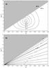 |
Fig. 2 For an assumed asteroid orbit typical of the Flora basin, namely a = 2.22 au, e = 0.1, the gray area at the top of both panels shows the region in the rotation frequency f = ω/ 2π and Δ plane, where the resonance zone about the Cassini state C2 does not exist for s = s6 = −26.34′′/yr frequency and I = I6 = 1.1° inclination. Conversely, the resonance zone exists in the white zone at the bottom of the panels. Top: for simplicity, we assume a Maxwellian distribution of f with a maximum probability density at 8 h rotation period (corresponding to the characteristics of large asteroids, e.g., Pravec et al. 2002), and a Gaussian distribution for the probability density of Δ, truncated and normalized to the definition interval 0 to 0.5, with a maximum at 0.25 and a standard deviation of 0.06 (roughly corresponding to typical asteroid shapes, e.g., Vokrouhlický & Čapek 2002). With these properties, the Cassini resonance characterized by | κ | >κ⋆ exists for 72% of cases. The isolines at the bottom of panel a) show regions of maximum probability density, with the label by the isoline depicting the total weight of the states enclosed by the curve in the white part of the graph. Bottom: using formulas given by Henrard & Murigande (1987), we calculate the area of the Cassini resonance zone about C2 on a unit sphere, normalized to its total area 4π, for each of the f and Δ combination in the plot (and other orbital parameters noted above). The isolines in panel b) show the result expressed in percents, indicating that the resonance zone typically covers ≃10% of the sphere. |
Generally speaking, the occurrence of any given rotation state of an asteroid in the resonant zone about the C2 state requires a fine-tuning of parameters and thus it is a priori unlikely, especially for low-inclination orbits or a resonance zone associated with Fourier term in ζ with a low value of amplitude Ai. This is because several constraints must be satisfied. First, we have seen that | κ | >κ⋆, which requires a correlated combination of the rotation frequency ω and the dynamical ellipticity parameter Δ from (2). The panels in Fig. 2 show the limited zone in the ω−Δ plane where | κ | >κ⋆. However, not all ω and Δ values are equally likely. For the sake of simplicity, we assumed an approximately Gaussian distribution of Δ values with a mean value of 0.25 and a standard deviation 0.06, roughly matching the data in Fig. 2 of Vokrouhlický & Čapek (2002). Additionally, we assumed a Maxwellian distribution of the rotational frequency f = ω/ 2π with a mean frequency of three cycles per day (e.g., Pravec et al. 2002), as is characteristic of large asteroids (larger than ≃20–30 km, which roughly corresponds to those observed by Kryszczyńska 2013). The isolines in the top panel of Fig. 2 show a combined probability density distribution function normalized to the whole ω−Δ plane. From this exercise, we estimate that the C2-associated resonance zone exists in ≃72% of cases for the following orbital parameters: a ≃ 2.22 au, e ≃ 0.1, I6 ≃ 1.1° and s6 ≃ −26.34′′/yr, typical of the Flora region. Even if this condition is satisfied, that is, if f and Δ happen to reside in the bottom white region of the plot, the orientation of s must fall into the resonance zone about C2. To estimate how likely this is to occur, we computed for each f and Δ value the angular area of the resonance using the analytical formulas given by Henrard & Murigande (1987; see also Hamilton & Ward 2004), and normalized them to the surface area of the whole unit sphere (i.e., 4π). If the rotation pole values of asteroids were isotropic in space, this surface area ratio would have been the probability estimate of a pole residence in the resonance (see bottom part of Fig. 2). For other pole-orientation distributions on the sky, one could run a Monte Carlo computation of this probability. However, we here adopted the simple area argument, noting that the general conclusions we draw from our test are not overly dependent on this simplification. Since the probabilities evaluated in the panels of Fig. 2, namely occurrence of the f and Δ values and pole residence in the resonant zone about C2, are independent, the total probability of finding a given asteroid from a sample with its pole captured in the Cassini resonance is a simple product of the two. We thus find that there is ~6% chance of this to happen. If we were to exclude the cases where the Cassini resonance about the C2 state of the proper frequency s also exists for low-inclination orbits in the Flora region (because it could produce a strong perturbation for the pole residence in the resonance Cassini zone corresponding to the s6 frequency), this probability would drop to ≃4%. Finding many asteroids in a given sample close to or in the resonance zone corresponding to the s6 frequency (as suggested by Kryszczyńska 2013) would therefore be a very unlikely situation.
Another aspect of studying a possibility for finding a rotation state of a given asteroid in the C2 state is analyzing the stability of its residence in the corresponding resonance zone. If the stability is high, one may imagine evolutionary scenarios that lead to a capture of the resonance in the past. If the resonance was an attractor of such evolutionary paths, and the post-capture residence in the resonance is stable, the overall probability of residing near C2 state may be much higher than estimated above. This is exactly the proposed scenario for existence of the Slivan states among the Koronis family members (e.g., Vokrouhlický et al. 2003). If, on the other hand, the stability is low, one should rely on the simple probability estimate of finding the spin state in the resonant zone at random. For these reasons, we examined the stability of the proposed Slivan states in the inner part of the main asteroid belt in Sect. 3. In Sect. 3.4 we also briefly examine the possibility of a capture into this state from a low-obliquity initial situation and a rotation period that increases as a result of the thermal torques.
2.2. Tools
In the next sections we numerically integrate Eq. (5) to investigate the secular spin axis evolution of selected asteroids in the inner part of the main belt. We make use of the efficient symplectic integrator proposed by Breiter et al. (2005), in particular, by adopting the LP2 splitting scheme. Since we deal with the secular evolution of s, we chose a conveniently long timestep of 50 yr. The code needs time series that describe the orbital evolution of the asteroid: the values of the semimajor axis a, the eccentricity e, and the complex parameter ζ that combines the longitude of the node and the inclination. This information was obtained using the well-tested and widely used integration package6swift. Because swift integrates the full system of equations of motion for both planets and asteroid(s), it requires an accordingly shorter timestep. We typically used 5 d, short enough to realistically describe the orbital evolution of all bodies (including Mercury). The initial orbital state vectors for the chosen asteroids and a given epoch were taken from the AstDyS internet database7, and for the planets from the JPL DE405 ephemerides file. To organize the propagation efficiently, we embedded our secular spin integration scheme into the swift package. This arrangement not only allowed us to propagate the spin evolution online, avoiding large output files with the orbital evolution, but it also allowed us to simultaneously propagate the spin evolution of more asteroids or parametric variants of the same asteroid (for instance, testing the evolution for different values of the dynamical ellipticity parameter Δ). Note that the spin propagation only needs at a given time to know the orbital parameters in the neighboring grid-points in time, which is readily provided by the swift integrator.
The numerical integration described above provides the time evolution of s with respect to the osculating orbital frame ℰ′. By applying the inverse matrix A-1 = AT, we may also obtain s in the inertial frame8ℰ. To understand the possible affinity of the spin vector to the Colombo top model concepts introduced above, we may now choose one of the Fourier terms in decomposition of ζ and transform s into a fictitious orbital frame ℰ′′ related to this particular term (as if it were the only one in ζ and the Colombo top model applied). Obviously, presence of other terms in ζ implies that the spin evolution in ℰ′′ does not exactly follow the flow-lines of the Colombo Hamiltonian (11), but if they represent only a small perturbation, the evolution would stay close to them. Since we are mainly interested in the occurrence of the Slivan states, we chose the forced term in ζ associated with the frequency s6 and constructed the associated reference frame ℰ′′.
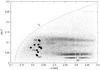 |
Fig. 3 Inner part of the asteroid main belt shown in projection onto the plane of the proper semimajor axis a and the proper sine of inclination sinI. Our working definition of the inner part is a< 2.5 au, the position of the 3/1 mean motion resonance with Jupiter, and we also exclude here the high-inclination population of Phocaeas. The dashed line indicates the approximate location of the ν6 secular resonance. Black symbols indicate prograde-rotating objects from the study of Kryszczyńska (2013), and the three objects discussed in Sect. 3 are labeled. The open symbol shows the location of (20) Massalia, the largest member of its own family. |
3. Flora region asteroids
To place the studied asteroids in context, we show in Fig. 3 their position in the space of proper orbital elements, semimajor axis a, and sine of inclination sinI, together with other asteroids in the inner part of the main belt. Synthetic proper elements were taken from the AstDyS website at the University of Pisa. While the ν6 secular resonance somewhat constrains the highest inclination values in the Flora region, some objects still have a proper inclination of up to ~7°. To demonstrate the fundamental role of the orbital inclination value, we selected three cases with different I values from the sample of bodies in Kryszczyńska (2013) and studied the stability of the spin axis confinement in the Slivan state for these bodies.
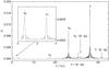 |
Fig. 4 Frequency spectrum of ζ = sin(I/ 2)exp(ıΩ) from a 10 Myr numerical orbital integration of (291) Alice. The abscissa is the frequency ν in arcseconds per year, and the ordinate in amplitude of the quasiperiodic approximation of ζ with Aexp [ı(νt + φ)]. The principal spectral lines are labeled with the standard notation in planetary studies: (i) s is the proper frequency; (ii) s6 is the principal planetary frequency due to the nodal precession of Saturn; (iii) s4, s7 and s8 are planetary frequencies with smaller amplitudes; and (iv) s ± (g−g6) are smaller nonlinear terms that also combine the perihelion proper and forced frequencies (due to the proximity of the ν6 secular resonance at the bottom of the main asteroid belt). |
3.1. Case of low inclination: (291) Alice
 |
Fig. 5 Evolution of the rotation pole for (291) Alice projected onto the reference frame ℰ′′ associated with the s6 frequency term in the Fourier representation of the ζ = sin(I/ 2)exp(ıΩ) orbital parameter (see Sect. 2.2). Four panels are shown for four values of the dynamical flattening parameter Δ. The dashed lines show a grid of meridian and latitude circles in ℰ′′ with the north pole toward the center and the zero longitude meridian, ϕ = 0°, pointing to the bottom of each figure (the viewing angle is similar to that of the bottom and left panel in Fig. 1). The solid lines are isolines of constant Colombo Hamiltonian ℋ′(X′,ϕ) = C for frequency s = s6 = −26.34′′/yr and inclination I = I6 = 1.1°. In the middle panels the spin remains well confined in the resonant zone about the Cassini state C2, in the extreme left and right panels the libration amplitude is larger and the perturbation due to the proper term in ζ brings the spin toward the limits of the Cassini resonance, indicating a possible long-term instability of the capture. |
We started with the case of the lowest inclination orbit in the sample, namely asteroid (291) Alice. Figure 4 shows a power spectrum of ζ = sin(I/ 2)exp(ıΩ) from a numerical integration spanning the time interval of 10 Myr. We used the algorithm by Ferraz-Mello (1981) that seeks to represent the signal with Fourier terms Aexp [ı(νt + φ)], optimizing A and φ by a least-squares method for a given frequency ν. We allowed a range of ν between −0.1′′/yr (set by the timespan of integration) and −100′′/yr (covering the expected signal reasonably well). The principal two lines in the spectrum are (i) the proper term with frequency s ≃ −36.44′′/yr and amplitude corresponding to an inclination IP ≃ 2.1°; and (ii) the forced term with frequency s6 ≃ −26.34′′/yr and amplitude corresponding to an inclination I6 ≃ 1.1°. The phase of the latter is φ6 ≃ 307°. Given the low inclinations of all terms, this renders the longitude of the Cassini state C2, that is, ϕ = 0° meridian of the corresponding reference frame ℰ′′, at about 37° ecliptic longitude. Other linear forced planetary terms, such as s4, s7 and s8 present in ζ have a significantly smaller amplitude and are of little importance. Thanks to proximity of the secular resonance ν6, g = g6 where g and g6 are the corresponding proper and forced frequencies in the longitude of perihelion, there are nonlinear secular terms such as s ± (g−g6) present in the spectrum of ζ. Their amplitude is limited, such that the contribution of the s and s6 terms dominates (see also Vokrouhlický et al. 2006c). In this case, the proper inclination value IP is only less than a factor 2 higher than the forced inclination I6.
We adopted the spin-state solution from Kryszczyńska (2013), which has a rotation period of 4.316011 h and two possible pole orientations, (λ,β) = (67° ± 8°,56° ± 6°) (pole P1) and (λ,β) = (250° ± 8°,56° ± 6°) (pole P2) with λ and β ecliptic longitude and latitude. This ambiguity is characteristic for a pole solution derived from optical photometry alone. In favorable conditions, additional data such as infrared photometry, adaptive optics imaging, or star occultations resolve the ambiguity in the pole solution (e.g., Ďurech et al. 2015). At the time of writing, however, asteroids from the sample of Kryszczyńska (2013) do not possess these additional datasets. We therefore followed the suggestion of Kryszczyńska (2013) that the P1 pole values of several asteroids in the same zone of orbital space in the Flora region are clustered in a similar way as those in the Koronis family and thus preliminarily adopted them as the correct ones while awaiting further techniques to verify them. We only note that independent spin solution for several asteroids from the sample of Kryszczyńska (2013), including (291) Alice, were obtained by Hanuš et al. (2011) from a partially overlapping dataset of dense light curves and an independent dataset of sparse photometric data. These solutions agree with Kryszczyńska (2013) within the quoted intervals of uncertainty.
The remaining unknown parameter necessary for determining the precession constant α in Eq. (2) is the dynamical flattening Δ. In principle, the light-curve inversion technique provides a generally correct shape model of the asteroid, which may not represent the smaller-scale topographic features well, however. Additionally, an estimation of Δ would require knowing the density distribution inside the body. As a result, the shape models associated with the light-curve inversion may only provide a Δ value to about 10–20% accuracy. For (291) Alice we downloaded models from the DAMIT database (Ďurech et al. 2010)9, based on solution of Hanuš et al. (2011). Assuming a constant bulk density distribution and using formulas from Dobrovolskis (1996), we obtained an estimate Δ ≃ 0.35.
We note that the resonant zone about the Cassini state C2 exists for Δ ≥ 0.3 (e.g., Fig. 2). Using the tools described in Sect. 2.2, we explored the spin axis evolution of Alice within the next 10 Myr for Δ spanning the interval 0.3 to 0.4 values. For a higher Δ value the resonant zone about the C2 state associated with the proper frequency emerges, and this produces a significant perturbation of the spin axis evolution of Alice, preventing residence in the Slivan state. A sample of results is shown in Fig. 5, where the 10 Myr trajectory of the spin evolution of Alice has been transformed into the reference frame ℰ′′ of the s6 precession term in the orbit. We found that the spin remains in the resonant zone about the Cassini state C2 only for a very narrow interval of Δ values in between 0.34 and 0.35 (Fig. 5). Outside this interval, the spin evolution over the monitored 10 Myr timespan generally drifts from the resonant zone, only regaining it at sparse time windows. This is clearly caused by perturbations by other contributing terms in the Fourier development of ζ (see discussion in Sect. 2.1), mostly by the proper term with a frequency s ≃ −36.44′′/yr and an amplitude about twice as large as I6. Our results thus show that even in this lowest inclination case a permanent capture in the Slivan state (resonance zone about C2 in the chosen ℰ′′ frame) is problematic.
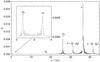 |
Fig. 6 Same as in Fig. 4, but now for asteroid (770) Bali. The spectrum is similar as above, but the amplitude of the proper term (proper inclination) is slightly larger. |
3.2. Case of medium inclination: (770) Bali
We now consider the case of (770) Bali, which has a slightly higher value of the proper inclination IP ≃ 3.6° (Fig. 6). While the general characteristics of the power spectrum of ζ are the same as for (291) Alice, the amplitude of the s ± (g−g6) sidebands of the proper frequency now increased. Because this asteroid resides in the nonlinear secular z2 resonance, the s ± 2(g−g6) creates an alias with the s6 contribution. Kryszczyńska (2013) provided pole solutions (λ,β) = (68° ± 5°,50° ± 5°) (pole P1) and (λ,β) = (262° ± 5°,45° ± 5°) (pole P2) for a sidereal rotation period of 5.818942 h. Again, a very similar solution has been reported by Hanuš et al. (2011). The shape model obtained from the light-curve inversion yields Δ ≃ 0.27.
Figure 7 shows the spin axis evolution of (770) Bali over a 10 Myr time interval projected onto the reference frame ℰ′′ of the s6 term in ζ for four values of Δ in a tight interval between 0.268 to 0.271. We note that the possibility of residing in the resonant state over the monitored interval of time now decreased to an even smaller range of Δ values, in spite of an only rather small change in proper inclination value.
3.3. Case of high inclination: (700) Auravictrix
Given the results from the previous sections, the prospects of a stable residence in the Cassini resonance for asteroids on still higher inclination orbits are weak at most. Indeed, we briefly analyzed the spin evolution for asteroid (700) Auravictrix, whose orbit has a proper inclination of IP ≃ 6.4°. The power spectrum of ζ indicates that not only the amplitude of the proper term now largely exceeds the amplitude of the s6 term, with still only an I6 ≃ 1.1° inclination, but the nonlinear sidebands with frequencies s ± (g−g6) now have a significant amplitude as well (Fig. 8). This is because with its higher inclination the asteroid resides closer to the ν6 resonance (Fig. 3). All this signal in ζ disrupts the stable libration in the Cassini resonant zone of the s6 frequency line.
Adopting the pole P1 solution from Kryszczyńska (2013), (λ,β) = (67° ± 10°,46° ± 6°) and a sidereal rotation period of 6.07484 h, we integrated the spin evolution of Auravictrix over the next 10 Myr interval of time. We considered a range of values for the flattening parameter Δ between 0.25 and 0.4. In none of the cases tested we observed a stable capture in the resonance zone around the Cassini state C2 associated with the s6 frequency. Figure 9 shows a few examples of the most promising choices of Δ for which the current pole resides at the formally low-amplitude isoline of the Colombo energy level ℋ′ = C. We note that even in these fine-tuned cases the pole exhibits strong deviations from the Cassini resonance zone. We were not able to find a case where the pole would remain localized inside the Slivan-resonance zone.
3.4. Capture in the Slivan state at low inclinations?
 |
Fig. 7 Same as in Fig. 5, but now for asteroid (770) Bali. Thanks to the higher value of the proper inclination (Fig. 6), perturbations of the spin evolution in the s6-frequency associated reference frame are now stronger. The stability of the librations about the C2 state is weaker as the solution tends to deviate from the resonant zone. |
Numerical simulations have shown that the affinity to the resonant zone of the Cassini state C2 is weak for asteroids in the Flora region. Yet, at least for the lowest inclination cases, we were able to find a range of Δ values for which the pole position mostly remained captured in the Slivan state over a 10 Myr interval of time. We now briefly analyze why the pole could be located in this state, since the results at the end of Sect. 2.1 suggested that a chance occurrence of this location has a rather low probability.
As indicated by the results in Vokrouhlický et al. (2003), a satisfactory possibility would be a capture from a low-obliquity state with the α parameter slowly evolving toward higher values. This can be caused in generally by decreasing the rotation frequency ω in the denominator of Eq. (2), or equivalently, by increasing the rotation period P. The Yarkovsky-O’Keefe-Radzievskii-Paddack (YORP) effect would be the first suspect for such a change in the rotation period of kilometer-sized asteroids (e.g., Bottke et al. 2006). For instance, considering (291) Alice with ≃12–13 km size, one might estimate a characteristic YORP timescale P/ (dP/ dt) ~ 500−700 Myr for a zero-obliquity state and P ≃ 6 h (see Čapek & Vokrouhlický 2004, for results and scaling laws). Thus Alice may have increased its rotation period from ~3 h to its current value of 4.32 h in perhaps less than a billion of years. This is about the estimated age of the Flora family (e.g., Nesvorný et al. 2002; Dykhuis et al. 2014), if indeed this asteroid is a member. Additionally, a billion-year timescale is shorter than the collisional lifetime of Alice-sized objects in the Flora region (e.g., Bottke et al. 2005). A similar estimate applies to the other asteroids in the sample of Kryszczyńska (2013).
Since here we are not interested in details of the possible past evolution due to the YORP effect, but merely we intend to explore the possibility of a past capture in the Slivan state, we restricted the formulation of the YORP effect to a simple past change in the rotation period. We first considered the case of (291) Alice with initially setting the rotation period to 3 h and letting it change with time at a constant rate dP/dt = 0.005 h/Myr (in fact, dω/dt rather than dP/dt should be constant, but we neglect this minor difference given the small change in P we are interested in). We assumed zero initial obliquity and Δ = 0.3464, for which results in Fig. 5 may promise a long-term lock in the Slivan state. Since for the initial P = 3 h we have | κ | <κ⋆ (interested in the s6 frequency mode), the Cassini resonance does not exist. The initial pole is close to the C2 equilibrium of the relevant Colombo model. As P increases, | κ | eventually reaches the critical value κ⋆, the resonant zone onsets at low obliquity and drifts to higher obliquities (eventually reaching the value ≃35° of C2 for the current rotation period of Alice; Fig. 5). If the evolution is slow enough (adiabatic, see Henrard & Murigande 1987), and perturbations from other spectral lines in ζ are kept low, the rotation pole could stay in the vicinity of the C2 equilibrium during the whole evolution.
Figure 10 shows the result of our simulation. In this case, the spin axis of Alice was successfully captured in the Slivan state and remained locked in this state till its rotation period reached the current value. Except for a slightly larger libration amplitude, the final spin state resembles our simulation from Fig. 5.
We repeated the same experiment for both (770) Bali and (700) Auravictrix. For Bali, we were again able to reproduce a capture in the Slivan state similar to what is shown in Fig. 10 for Alice. This is encouraging, although obviously the downside is that this only occurs for a very narrow range of Δ parameters, as shown in Fig. 7. As expected, no capture in the Slivan state was recorded for Auravictrix.
4. Massalia region asteroids
The innermost part of the main asteroid belt is not a favorable zone to expect an existence of the Slivan states. However, we now show that a niche can be found in the inner part of the belt where this interesting situation may be expected. Given our results so far, we focus on a region of the orbital space that (i) adheres to the 3/1 mean motion resonance with Jupiter; and (ii) has low inclinations. Figure 3 indicates that the asteroid population in this part of the phase space is dominated by several asteroid families (see also Nesvorný et al. 2015). The most prominent are the Massalia family and the Nysa-Hertha-Polana-Eulalia complex. The Euterpe cratering family might similarly be of interest, whose members have unusually low inclination orbits such that I6>IP in this case. We use Massalia as an example.
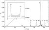 |
Fig. 8 Same as in Fig. 4, but now for asteroid (700) Auravictrix. The proper term, with the ± (g−g6) side-lines, now dominates and the contribution of s6 term is weaker. |
Figure 11 shows the power spectrum of ζ for (20) Massalia, representative for many members in its own family. Since the value of the semimajor axis is higher than in the Flora region, the proper frequency s has now increased to ≃−45.11′′/yr. This causes it to be better separated from the s6 frequency. The proper inclination is suitably low IP ≃ 1.4°, while the forced inclination of the s6 term remains I6 ≃ 0.9°. These two lines now dominate the Fourier representation of ζ, with only a very minor role played by contribution from other lines.
As an example we considered the pole solution for (20) Massalia from Kaasalainen et al. (2002), updated on the DAMIT website: (λ,β) = (0°,40°) (pole P1) and (λ,β) = (179°,39°) (pole P2) with a rotation period of 8.09902 h. The formal uncertainty of longitude and latitude values is ≃5°, but given the imperfect fit of the light-curve data, the realistic uncertainty might be slightly larger. While interesting, we use this asteroid’s data as an example of a possible spin evolution of members in its family. As a result, the uncertainties in its pole solutions are not critical for our conclusions. For that reason, the Δ value of ≃0.3 derived from the (20) Massalia shape solution at the DAMIT website is not critical for our considerations either (on top of the fact that this value might have a realistic uncertainty ≃0.05).
Figure 12 shows examples of a 10 Myr pole evolution of Massalia projected onto the reference frame ℰ′′ of the s6 frequency for four different values of the Δ parameter in a rather wide range from 0.22 to 0.32. In all cases, the pole performs a stable libration about the C2 stationary solution, following the isolines of constant Hamiltonian ℋ′ = C of the Colombo model rather closely. This is because the proper term in ζ now represents only a high-frequency and small-amplitude perturbation in ℰ′′. Clearly, stable Slivan states can exist among the Massalia family members. The particular case of (20) Massalia itself is interesting. Our simulation indicates that this asteroid might have its spin in the Slivan state. If confirmed, it might be considered as an example of the few percent fluke case (see discussion in Sect. 2.1), because this asteroid is too large to assume YORP evolution on any reasonable timescale. Additionally, according to Vokrouhlický et al. (2006a), the Massalia-family parent body underwent a large cratering event some 150–200 Myr ago, when the family has been formed, giving even less time for any evolution of (20) Massalia pole.
 |
Fig. 9 Same as in Fig. 5, but now for asteroid (700) Auravictrix. In this case, we only show a short time-segment from out 10 Myr numerical integration spanning 500 kyr. This is because plotting the whole output of the 10 Myr integration would just chaotically saturate the plot with pole positions. The open symbol shows the current pole location. |
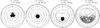 |
Fig. 10 Example of a successful capture of the spin axis of Alice in the Slivan state. The simulation assumed an initial rotation period of 3 h, the pole location at nearly zero obliquity, and Δ = 0.3464. For the sake of simplicity, the orbital evolution is represented by a numerical simulation of Alice from the current epoch. Each of the four panels shows a selected evolution of the pole in the 10 Myr duration window projected onto the frame associated with the s6 Fourier term in the orbital ζ: the leftmost panel shows the situation at the beginning of the simulation, the rightmost panel shows the situation at the end of the simulation. The top label also indicates the mean rotation period in the 10 Myr interval shown. |
Unfortunately, not much is currently known about the pole distribution of smaller members of the Massalia family. This is because the largest of them only have ≃(3–5) km in size at most. Interestingly, given the younger age of the Massalia family, the pole evolutionary tracks of its largest members may be similar to those of ≃(20–30) km size members in the ≃(2–3) Gyr old Koronis family. Consequently, we might expect that numerous Slivan states exist among the prograde-rotating Massalia members. Approximate methods allowing constraining the ecliptic longitude of the asteroid pole, such as in Bowell et al. (2014), may provide first hints.
5. Conclusion
We studied the possibility of an occurrence of Slivan states in the inner zone of the main asteroid belt. Our work has been motivated by recent results of Kryszczyńska (2013), who suggested the existence of such spin states for several members in the Flora region. However, we found this conclusion to be problematic, at least for bodies with a proper value of the orbital inclination higher than ≃4° (as for (700) Auravictrix discussed in Sect. 3.3). This is because the confinement in the Slivan state is too strongly perturbed by the proper-term contribution in the Fourier representation of orbital ζ. For objects with a proper value of the orbital inclination lower than ≃4° ((291) Alice and (770) Bali discussed in Sects. 3.1 and 3.2), a spin state that is long-term stable in the Slivan state is possible. Additionally, in these cases we also verified that the capture scenario proposed by Vokrouhlický et al. (2003) may explain the current Slivan state for these asteroids on a reasonable timescale of ~1 Gyr. However, the caveat here is that this only works for a very narrow interval of the Δ parameter. There is no reason why all the observed Flora asteroids would have just the correct values of this parameter to match the condition of residence in the respective Slivan state. While not fully satisfactory, the situation is interesting because it provides a double motivation for future work: (i) on the theoretical side, our analysis may be missing some important element that would need to be added to fully explain the situation; or/and (ii) on the observational side, it would be interesting to know more about the spin states of small Flora-region asteroids and understand in more detail which fraction may be near the Slivan state.
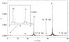 |
Fig. 11 Same as in Fig. 4, but now for asteroid (20) Massalia. Thanks to the higher value of the semimajor axis, a ≃ 2.41 au, the proper frequency s is now better separated from the forced frequency s6. These two lines now dominate the power spectrum of ζ for this asteroid. |
 |
Fig. 12 Same as in Fig. 5, but now for asteroid (20) Massalia. In this case, the stable residence in the Slivan state is possible for a wide range of Δ values: the leftmost and rightmost panels show approximately the limiting cases for the current spin state of Massalia. For the nominal Δ ≃ 0.3 value, the pole of Massalia would librate about the C2 state with about 80° amplitude. The open symbol shows the current P1 pole location (all integrations assumed this pole as the starting condition). |
As an example of (i), we may mention the following speculation, for instance. We have mentioned in Sect. 3.2 that the asteroid (770) Bali is located in the weak, nonlinear secular resonance z2 (e.g., Milani & Knežević 1994). Similarly, (700) Auravictrix is very close, but not in the z2 resonance. Given its secular nature, this structure has a complicated tilted shape in the space of proper orbital elements, extending from a lower a and I value towards higher a and I values in the Flora region. Prograde-rotating asteroids migrating outward as a result of the Yarkovsky effect may “slide” along the z2 resonance roughly from the location of (770) Bali to the location of (700) Auravictrix (see Fig. 3). Such a dynamical pathway has been discussed for small members in the Eos family, for instance (e.g., Vokrouhlický et al. 2006b). It is thus conceivable that (700) Auravictrix has recently been released from the z2 resonance after spending hundreds of Myr in it and originating at lower a and I state, where its spin axis could have been captured in the Slivan state. Demonstrating this possibility is beyond the scope of this paper, however.
A much more favorable situation for existence of Slivan states in the inner part of the asteroid belt occurs for asteroids residing on low-I orbits near the 3/1 mean motion resonance with Jupiter. Examples might be found among asteroids in the Massalia, Eulalia, or new Polana families after observations will allow solving their spin states.
The Cassini equilibria probably represent evolutionary end-states of numerous regular satellites, including our Moon (e.g., Gladman et al. 1996; Peale 1999), and even planets (e.g., Colombo 1966; Ward 1975; Ward & Hamilton 2004; Hamilton & Ward 2004; Peale 2006), and they are thus significant for understanding the long-term spin evolution of bodies in planetary systems. Nevertheless, applications to asteroid spin states were limited so far (e.g., Skoglöv et al. 1996; Skoglöv 1997, 1998; Vokrouhlický et al. 2005).
An exact identification of the Flora family membership is complicated by the significant dynamical chaoticity and high density of asteroids in the inner main-belt. For that reason, some of the asteroids in the sample of Kryszczyńska (2013) that were claimed to be members of the Flora family were not considered to belong to it by other researchers. For instance, the latest work of Nesvorný et al. (2015) did not assume asteroids on the lowest inclination orbits (e.g., (291) Alice or (367) Amicitia) to belong to this family. This ambiguity, however, does not affect our conclusions.
We recall that the longitude ϕ is measured in the orbital plane of the asteroid with an origin at a 90° angle from the ascending node.
For historical reasons these stationary solutions are called Cassini states (e.g., Colombo 1966).
Note that κ⋆ from Eq. (12) is positive by definition, while κ is typically negative, reflecting retrograde precession of the asteroid’s orbital plane, hence s< 0.
The integration scheme of Breiter et al. (2005) explicitly uses this transformation of s to the inertial frame in the midstep of the propagation.
Acknowledgments
This work was supported by the Czech Science Foundation (grant GA13-01308S) and project SVV-260089 of the Charles University. We thank the referee, whose suggestions helped to improve the submitted version of this paper.
References
- Bertotti, B., Farinella, P., & Vokrouhlický, D. 2003, Physics of the Solar System – Dynamics and Evolution, Space Physics, and Spacetime Structure (Dordrecht: Kluwer Academic Press) [Google Scholar]
- Bottke, W. F., Durda, D. D., Nesvorný, D., et al. 2005, Icarus, 179, 63 [NASA ADS] [CrossRef] [Google Scholar]
- Bottke, Jr., W. F., Vokrouhlický, D., Rubincam, D. P., & Nesvorný, D. 2006, Ann. Rev. Earth Planet. Sci., 34, 157 [Google Scholar]
- Bowell, E., Oszkiewicz, D. A., Wasserman, L. H., et al. 2014, Meteor. Planet. Sci., 49, 95 [NASA ADS] [CrossRef] [Google Scholar]
- Breiter, S., Nesvorný, D., & Vokrouhlický, D. 2005, AJ, 130, 1267 [NASA ADS] [CrossRef] [Google Scholar]
- Colombo, G. 1966, AJ, 71, 891 [NASA ADS] [CrossRef] [Google Scholar]
- Dobrovolskis, A. R. 1996, Icarus, 124, 698 [NASA ADS] [CrossRef] [Google Scholar]
- Ďurech, J., Sidorin, V., & Kaasalainen, M. 2010, A&A, 513, A46 [NASA ADS] [CrossRef] [EDP Sciences] [Google Scholar]
- Ďurech, J., Carry, B., Delbò, M., Kaasalainen, M., & Viikinkoski, M. 2015, in Asteroids IV, eds. P. Michel, F. E. DeMeo, & W. F. Bottke [Google Scholar]
- Dykhuis, M. J., Molnar, L., Van Kooten, S. J., & Greenberg, R. 2014, Icarus, 243, 111 [NASA ADS] [CrossRef] [Google Scholar]
- Ferraz-Mello, S. 1981, AJ, 86, 619 [NASA ADS] [CrossRef] [Google Scholar]
- Gladman, B., Quinn, D. D., Nicholson, P., & Rand, R. 1996, Icarus, 122, 166 [NASA ADS] [CrossRef] [Google Scholar]
- Hamilton, D. P., & Ward, W. R. 2004, AJ, 128, 2510 [NASA ADS] [CrossRef] [Google Scholar]
- Hanuš, J., Ďurech, J., Brož, M., et al. 2011, A&A, 530, A134 [NASA ADS] [CrossRef] [EDP Sciences] [Google Scholar]
- Henrard, J., & Murigande, C. 1987, Celestial Mechanics, 40, 345 [NASA ADS] [CrossRef] [Google Scholar]
- Kaasalainen, M., Torppa, J., & Piironen, J. 2002, Icarus, 159, 369 [NASA ADS] [CrossRef] [Google Scholar]
- Kryszczyńska, A. 2013, A&A, 551, A102 [NASA ADS] [CrossRef] [EDP Sciences] [Google Scholar]
- Kryszczyńska, A., Colas, F., Polińska, M., et al. 2012, A&A, 546, A72 [NASA ADS] [CrossRef] [EDP Sciences] [Google Scholar]
- Laskar, J., & Robutel, P. 1993, Nature, 361, 608 [NASA ADS] [CrossRef] [Google Scholar]
- Milani, A., & Knežević, Z. 1994, Icarus, 107, 219 [NASA ADS] [CrossRef] [Google Scholar]
- Neron de Surgy, O., & Laskar, J. 1997, A&A, 318, 975 [NASA ADS] [Google Scholar]
- Nesvorný, D., Morbidelli, A., Vokrouhlický, D., Bottke, W. F., & Brož, M. 2002, Icarus, 157, 155 [NASA ADS] [CrossRef] [Google Scholar]
- Nesvorný, D., Brož, M., & Carruba, V. 2015, in Astroids VI, eds. P. Michel et al. (University of Arizona Press), in press [arXiv:1502.01628] [Google Scholar]
- Peale, S. J. 1999, ARA&A, 37, 533 [NASA ADS] [CrossRef] [Google Scholar]
- Peale, S. J. 2006, Icarus, 181, 338 [NASA ADS] [CrossRef] [Google Scholar]
- Pravec, P., Harris, A. W., & Michalowski, T. 2002, in Asteroids III, eds. W. F. Bottke, A. Cellino, P. Paolicchi, & R. P. Binzel, 113 [Google Scholar]
- Skoglöv, E. 1997, Planet. Space Sci., 45, 439 [Google Scholar]
- Skoglöv, E. 1998, Planet. Space Sci., 47, 11 [NASA ADS] [CrossRef] [Google Scholar]
- Skoglöv, E., Magnusson, P., & Dahlgren, M. 1996, Planet. Space Sci., 44, 1177 [NASA ADS] [CrossRef] [Google Scholar]
- Slivan, S. M. 2002, Nature, 419, 49 [Google Scholar]
- Slivan, S. M., Binzel, R. P., Kaasalainen, M., et al. 2009, Icarus, 200, 514 [NASA ADS] [CrossRef] [Google Scholar]
- Čapek, D., & Vokrouhlický, D. 2004, Icarus, 172, 526 [NASA ADS] [CrossRef] [Google Scholar]
- Vokrouhlický, D., & Čapek, D. 2002, Icarus, 159, 449 [NASA ADS] [CrossRef] [Google Scholar]
- Vokrouhlický, D., Nesvorný, D., & Bottke, W. F. 2003, Nature, 425, 147 [NASA ADS] [CrossRef] [PubMed] [Google Scholar]
- Vokrouhlický, D., Bottke, W. F., & Nesvorný, D. 2005, Icarus, 175, 419 [NASA ADS] [CrossRef] [Google Scholar]
- Vokrouhlický, D., Brož, M., Bottke, W. F., Nesvorný, D., & Morbidelli, A. 2006a, Icarus, 182, 118 [NASA ADS] [CrossRef] [Google Scholar]
- Vokrouhlický, D., Brož, M., Morbidelli, A., et al. 2006b, Icarus, 182, 92 [NASA ADS] [CrossRef] [Google Scholar]
- Vokrouhlický, D., Nesvorný, D., & Bottke, W. F. 2006c, Icarus, 184, 1 [NASA ADS] [CrossRef] [Google Scholar]
- Ward, W. R. 1975, AJ, 80, 64 [NASA ADS] [CrossRef] [Google Scholar]
- Ward, W. R., & Hamilton, D. P. 2004, AJ, 128, 2501 [NASA ADS] [CrossRef] [Google Scholar]
All Figures
|
Fig. 1 Isolines ℋ′ = C on a unit sphere for the Colombo top model with I = 5° and κ = −0.914; since | κ | >κ⋆ ≃ 0.652 there are four stationary (Cassini) equilibria of the flow denoted by symbols and labeled C1 to C4. The resonant zone about C2 is highlighted by gray shading. The four panels show different angles of view; the coordinate grid is such that colatitude ε is measured from the north pole near C1, and the longitude ϕ is measured from the meridian of the C2 equilibrium. |
| In the text | |
|
Fig. 2 For an assumed asteroid orbit typical of the Flora basin, namely a = 2.22 au, e = 0.1, the gray area at the top of both panels shows the region in the rotation frequency f = ω/ 2π and Δ plane, where the resonance zone about the Cassini state C2 does not exist for s = s6 = −26.34′′/yr frequency and I = I6 = 1.1° inclination. Conversely, the resonance zone exists in the white zone at the bottom of the panels. Top: for simplicity, we assume a Maxwellian distribution of f with a maximum probability density at 8 h rotation period (corresponding to the characteristics of large asteroids, e.g., Pravec et al. 2002), and a Gaussian distribution for the probability density of Δ, truncated and normalized to the definition interval 0 to 0.5, with a maximum at 0.25 and a standard deviation of 0.06 (roughly corresponding to typical asteroid shapes, e.g., Vokrouhlický & Čapek 2002). With these properties, the Cassini resonance characterized by | κ | >κ⋆ exists for 72% of cases. The isolines at the bottom of panel a) show regions of maximum probability density, with the label by the isoline depicting the total weight of the states enclosed by the curve in the white part of the graph. Bottom: using formulas given by Henrard & Murigande (1987), we calculate the area of the Cassini resonance zone about C2 on a unit sphere, normalized to its total area 4π, for each of the f and Δ combination in the plot (and other orbital parameters noted above). The isolines in panel b) show the result expressed in percents, indicating that the resonance zone typically covers ≃10% of the sphere. |
| In the text | |
|
Fig. 3 Inner part of the asteroid main belt shown in projection onto the plane of the proper semimajor axis a and the proper sine of inclination sinI. Our working definition of the inner part is a< 2.5 au, the position of the 3/1 mean motion resonance with Jupiter, and we also exclude here the high-inclination population of Phocaeas. The dashed line indicates the approximate location of the ν6 secular resonance. Black symbols indicate prograde-rotating objects from the study of Kryszczyńska (2013), and the three objects discussed in Sect. 3 are labeled. The open symbol shows the location of (20) Massalia, the largest member of its own family. |
| In the text | |
|
Fig. 4 Frequency spectrum of ζ = sin(I/ 2)exp(ıΩ) from a 10 Myr numerical orbital integration of (291) Alice. The abscissa is the frequency ν in arcseconds per year, and the ordinate in amplitude of the quasiperiodic approximation of ζ with Aexp [ı(νt + φ)]. The principal spectral lines are labeled with the standard notation in planetary studies: (i) s is the proper frequency; (ii) s6 is the principal planetary frequency due to the nodal precession of Saturn; (iii) s4, s7 and s8 are planetary frequencies with smaller amplitudes; and (iv) s ± (g−g6) are smaller nonlinear terms that also combine the perihelion proper and forced frequencies (due to the proximity of the ν6 secular resonance at the bottom of the main asteroid belt). |
| In the text | |
|
Fig. 5 Evolution of the rotation pole for (291) Alice projected onto the reference frame ℰ′′ associated with the s6 frequency term in the Fourier representation of the ζ = sin(I/ 2)exp(ıΩ) orbital parameter (see Sect. 2.2). Four panels are shown for four values of the dynamical flattening parameter Δ. The dashed lines show a grid of meridian and latitude circles in ℰ′′ with the north pole toward the center and the zero longitude meridian, ϕ = 0°, pointing to the bottom of each figure (the viewing angle is similar to that of the bottom and left panel in Fig. 1). The solid lines are isolines of constant Colombo Hamiltonian ℋ′(X′,ϕ) = C for frequency s = s6 = −26.34′′/yr and inclination I = I6 = 1.1°. In the middle panels the spin remains well confined in the resonant zone about the Cassini state C2, in the extreme left and right panels the libration amplitude is larger and the perturbation due to the proper term in ζ brings the spin toward the limits of the Cassini resonance, indicating a possible long-term instability of the capture. |
| In the text | |
|
Fig. 6 Same as in Fig. 4, but now for asteroid (770) Bali. The spectrum is similar as above, but the amplitude of the proper term (proper inclination) is slightly larger. |
| In the text | |
|
Fig. 7 Same as in Fig. 5, but now for asteroid (770) Bali. Thanks to the higher value of the proper inclination (Fig. 6), perturbations of the spin evolution in the s6-frequency associated reference frame are now stronger. The stability of the librations about the C2 state is weaker as the solution tends to deviate from the resonant zone. |
| In the text | |
|
Fig. 8 Same as in Fig. 4, but now for asteroid (700) Auravictrix. The proper term, with the ± (g−g6) side-lines, now dominates and the contribution of s6 term is weaker. |
| In the text | |
|
Fig. 9 Same as in Fig. 5, but now for asteroid (700) Auravictrix. In this case, we only show a short time-segment from out 10 Myr numerical integration spanning 500 kyr. This is because plotting the whole output of the 10 Myr integration would just chaotically saturate the plot with pole positions. The open symbol shows the current pole location. |
| In the text | |
|
Fig. 10 Example of a successful capture of the spin axis of Alice in the Slivan state. The simulation assumed an initial rotation period of 3 h, the pole location at nearly zero obliquity, and Δ = 0.3464. For the sake of simplicity, the orbital evolution is represented by a numerical simulation of Alice from the current epoch. Each of the four panels shows a selected evolution of the pole in the 10 Myr duration window projected onto the frame associated with the s6 Fourier term in the orbital ζ: the leftmost panel shows the situation at the beginning of the simulation, the rightmost panel shows the situation at the end of the simulation. The top label also indicates the mean rotation period in the 10 Myr interval shown. |
| In the text | |
|
Fig. 11 Same as in Fig. 4, but now for asteroid (20) Massalia. Thanks to the higher value of the semimajor axis, a ≃ 2.41 au, the proper frequency s is now better separated from the forced frequency s6. These two lines now dominate the power spectrum of ζ for this asteroid. |
| In the text | |
|
Fig. 12 Same as in Fig. 5, but now for asteroid (20) Massalia. In this case, the stable residence in the Slivan state is possible for a wide range of Δ values: the leftmost and rightmost panels show approximately the limiting cases for the current spin state of Massalia. For the nominal Δ ≃ 0.3 value, the pole of Massalia would librate about the C2 state with about 80° amplitude. The open symbol shows the current P1 pole location (all integrations assumed this pole as the starting condition). |
| In the text | |
Current usage metrics show cumulative count of Article Views (full-text article views including HTML views, PDF and ePub downloads, according to the available data) and Abstracts Views on Vision4Press platform.
Data correspond to usage on the plateform after 2015. The current usage metrics is available 48-96 hours after online publication and is updated daily on week days.
Initial download of the metrics may take a while.