© ESO, 2015

1. Introduction

The majority of the plasma-physics literature on shocks essentially considers general flux-conservation requirements only, leading to the well-known Rankine-Hugoniot relations (e.g., see Serrin 1959; Hudson 1970; Baumjohann & Treumann 1996; Gombosi 1998; Diver 2001). These relations, however, do not explicitly formulate the internal microphysical processes that generate internal entropy during the conversion from the upstream regime into the downstream plasma. The missing physics in this description evidently leads to the well-known phenomenon that the set of Rankine-Hugoniot relations is a mathematically unclosed system of equations. Therefore, these relations can only provide unequivocal solutions if additional physical relations are added to the system, such as the assumption of an adiabatic reaction of the plasma ions during their compression into the higher-density regime on the downstream side (e.g., Erkaev et al. 2000).

The solar-wind termination shock is a particular example of a plasma shock for which microphysical effects play an important role. According to recent studies, pick-up ions have a crucial influence on overall shock physics at the solar-wind termination shock. They are a thermodynamically important additional plasma component, since they extract a significant fraction of the upstream kinetic energy in the form of thermal energy at the termination shock (see Decker et al. 2008). Zank et al. (2010) and Fahr & Siewert (2007, 2010, 2011) have studied kinetic features of this multicomponent shock transition and found relations between upstream and downstream ion distribution functions that are different for solar-wind protons and pick-up protons. Although these studies discuss the required overadiabatic reaction of pick-up ions, a satisfying explanation of all plasma properties observed by Voyager-2 (Richardson et al. 2008) is still lacking as demonstrated by Chalov & Fahr (2013). The latter authors show that assuming a significant difference in the behavior of solar-wind electrons compared to protons, namely as an independent plasma fluid, leads to an explanation of most of the observed plasma data presented by Richardson et al. (2008) in a satisfying manner.

To achieve this result in their parameterized study, Chalov & Fahr (2013) had to include preferential heating of the solar-wind electrons during the shock passage by a factor of about ten stronger than the proton heating. This type of electron heating at the potential jump of fast-mode shocks had been realized earlier by Leroy & Mangeney (1984), Tokar et al. (1986), and Schwartz et al. (1988), and the phenomenon of shock-heated electrons also appears in plasma-shock simulations when electrons are treated kinetically (see Lembège et al. 2003, 2004). In these cases, the plasma electrons demagnetize due to two-stream and viscous interactions and attain downstream-to-upstream temperature ratios of 50 and more.

Leroy et al. (1982) and Goodrich & Scudder (1984) follow a different approach. In their treatments, the plasma electrons carry drifts perpendicular to the shock normal (z-direction) different from the ion motion as a reaction to the shock-electric field. These drifts establish an electric current j_⊥, which is responsible for the change of the surface parallel magnetic field B_∥ in the form 4πj_⊥/c = dB_∥/ dz. To achieve the same consistency, Fahr et al. (2012) describe the conditions of the upstream and downstream plasma in the bulk frame systems with a frozen-in magnetic field. In this framework, the Liouville-Vlasov theorem describes all relevant downstream plasma quantities as an instantaneous kinetic reaction in the velocity distribution function during the transition from upstream to downstream. The excessive electron heating is then the result of the mass- and charge-specific reactions to the electric shock ramp, as shown in the semikinetic models of the multifluid termination shock by Fahr et al. (2012) and Fahr & Siewert (2013). According to these studies, electrons enter the downstream side as a strongly heated plasma fluid with negligible mass density that dominates the downstream plasma pressure.

In this paper, we demonstrate why the Voyager-1/-2 spacecraft did not detect these theoretically suggested hot electrons (see Richardson et al. 2008) when they penetrated into the heliosheath plasma. For the purpose of clarification, we analyze the downstream plasma conditions in more detail under which the detection of preferentially heated electrons would have to take place.

2. Theoretical description of downstream electrons

In the following section, we shall start from a theoretical description of solar-wind electrons expected downstream of the termination shock (Fahr & Siewert 2013). We treat them as a separate plasma species, which reacts in a very specific manner to the electric-field structure connected with the shock before adapting to the downstream plasma bulk frame. In the shock-at-rest system, the shock electric potential ramp decelerates the upstream protons from the upstream bulk velocity U₁ to the downstream bulk velocity U_2,p, which is comparable to the center-of-mass flow ${\mathit{U}}_{\mathrm{2}}^{\mathrm{\ast }}\mathrm{\simeq }{\mathit{U}}_{\mathrm{2}\mathit{,}\mathrm{p}}\mathrm{(}\mathrm{1}\mathrm{+}\mathit{s}\sqrt{\mathit{m}\mathit{/}\mathit{M}}\mathrm{)}$, where s is the shock compression ratio and m,M denote the masses of electrons and protons, respectively. The downstream magnetic field is frozen-in into the center-of-mass flow, and all plasma components are eventually comoving with the center-of-mass flow (Chashei & Fahr 2013). The electrons, on the other hand, react in a completely different way to this electric potential. First, they attain a strong “overshoot” velocity U_2,e which then relaxes rapidly to the center-of-mass bulk velocity ${\mathit{U}}_{\mathrm{2}}^{\mathrm{\ast }}$ enforced by the frozen-in magnetic field. During this relaxation process, the plasma generates randomized thermal velocity components through the action of the two-stream instability or the Buneman instability as well as by pitch-angle scattering (see Chashei & Fahr 2013, 2014; Fahr et al. 2014).

Under the assumptions of an instantaneous reaction of the electrons to the electric potential and randomization of the overshoot energy by the Buneman instability and pitch-angle scattering to an isotropic distribution in the downstream bulk frame, we obtain (Fahr & Siewert 2013, 2015) the following expression for the electron pressure P_2,e on the downstream-side of the shock: ${\mathit{P}}_{\mathrm{2}\mathit{,}\mathrm{e}}\mathrm{=}\frac{\mathit{M}}{\mathit{m}}\frac{{\mathit{s}}^{\mathrm{2}}\mathrm{-}\mathrm{1}}{\mathit{s}}\frac{{\mathit{U}}_{\mathrm{1}}^{\mathrm{2}}}{{\mathit{c}}_{\mathrm{1}\mathit{,}\mathrm{e}}^{\mathrm{2}}}\mathrm{\left[}\mathit{A}\mathrm{\right(}\mathit{\alpha }\mathrm{)}{\sin }^{\mathrm{2}}\mathit{\alpha }\mathrm{+}\mathit{B}\mathrm{(}\mathit{\alpha }\mathrm{)}{\cos }^{\mathrm{2}}{\mathit{\alpha }}^{\mathrm{]}}{\mathit{P}}_{\mathrm{1}\mathit{,}\mathrm{p}}\mathit{.}$(1)The indices p and e denote proton- or electron-relevant quantities, and the indices 1 and 2 denote upstream and downstream quantities, respectively. The parameter U denotes the bulk velocity, and s is the shock compression ratio. The parameter c_1,e is the average electron thermal velocity on the upstream side, where we assume that solar-wind electrons and protons have equal temperatures. We denote the magnetic tilt angle between the shock normal and the upstream magnetic field as α. The functions A(α) and B(α) are given in Fahr & Siewert (2013). In the limit of vanishing thermal pressures and dominating magnetic pressures, the self-consistent compression ratio s turns out to be s = 1 (see Fahr & Siewert 2013, Eq. (18)). Instead of treating the calculated velocity moment P_2,e of the distribution function, we focus on the distribution function f_2,e itself to derive the expected electron particle fluxes g_2,e as the relevant observable for the Voyager-1/-2 instrumentation. As motivated in Fahr & Siewert (2013), we assume that the downstream nonequilibrium distribution function f_2,e is a general kappa-distribution. This convenient choice represents the transition from a thermal core to a suprathermal tail distribution. The kappa-distribution is given by ${\mathit{f}}_{\mathrm{e}}\mathrm{\left(}\mathit{v}\mathrm{\right)}\mathrm{=}\frac{{\mathit{n}}_{\mathrm{e}}}{{\mathit{\pi }}^{\mathrm{3}\mathit{/}\mathrm{2}}{\mathit{\kappa }}_{\mathrm{e}}^{\mathrm{3}\mathit{/}\mathrm{2}}{\mathrm{\Theta }}_{\mathrm{e}}^{\mathrm{3}}}\frac{\mathrm{\Gamma }\mathrm{(}{\mathit{\kappa }}_{\mathrm{e}}\mathrm{+}\mathrm{1}\mathrm{)}}{\mathrm{\Gamma }\mathrm{(}{\mathit{\kappa }}_{\mathrm{e}}\mathrm{-}\mathrm{1}\mathit{/}\mathrm{2}\mathrm{)}}{\left[\mathrm{1}\mathrm{+}\frac{{\mathit{v}}^{\mathrm{2}}}{{\mathit{\kappa }}_{\mathrm{e}}{\mathrm{\Theta }}_{\mathrm{e}}^{\mathrm{2}}}\right]}^{\mathrm{-}\left({\mathit{\kappa }}_{\mathrm{e}}\mathrm{+}\mathrm{1}\right)}\mathit{,}$(2)where n_e is the electron number density, Θ_e is the velocity width of the thermal core, and κ_e is the specific electron kappa parameter with a range of 3/2 ≤ κ_2,e, ≤ ∞. The symbol Γ = Γ(x) denotes the Gamma function of the argument x.

In the next step, we determine the adequate value of κ_2,e for electrons downstream of the shock associated with a pressure given by Eq. (1). For this purpose, we determine the associated pressure P_2,e,κ (i.e., the pressure resulting as the second velocity moment of the above distribution, Eq. (2), see Heerikhuisen et al. 2008) that is equal to the pressure given by Eq. (1) (i.e., the electron pressure found in the multifluid approach by Fahr & Siewert 2013). We obtain the following relation for P_2,e,κ: $\begin{array}{ccc}{\mathit{P}}_{\mathrm{2}\mathit{,}\mathrm{e}\mathit{,\kappa }}\mathrm{\left(}\mathit{\kappa }\mathrm{\right)}& \mathrm{=}& {\mathit{n}}_{\mathrm{2}\mathit{,}\mathrm{e}}\frac{\mathit{m}}{\mathrm{2}}{\mathrm{\Theta }}_{\mathrm{2}\mathit{,}\mathrm{e}}^{\mathrm{2}}\frac{{\mathit{\kappa }}_{\mathrm{2}\mathit{,}\mathrm{e}}}{{\mathit{\kappa }}_{\mathrm{2}\mathit{,}\mathrm{e}}\mathrm{-}\mathrm{3}\mathit{/}\mathrm{2}}\\ & \mathrm{=}& \frac{\mathit{M}}{\mathit{m}}\frac{{\mathit{s}}^{\mathrm{2}}\mathrm{-}\mathrm{1}}{\mathit{s}}\frac{{\mathit{U}}_{\mathrm{1}}^{\mathrm{2}}}{{\mathit{c}}_{\mathrm{1}\mathit{,}\mathrm{e}}^{\mathrm{2}}}\mathrm{\left[}\mathit{A}\mathrm{\right(}\mathit{\alpha }\mathrm{)}{\sin }^{\mathrm{2}}\mathit{\alpha }\mathrm{+}\mathit{B}\mathrm{(}\mathit{\alpha }\mathrm{\left)}{\cos }^{\mathrm{2}}\mathit{\alpha }\mathrm{\right]}{\mathit{P}}_{\mathrm{1}\mathit{,}\mathrm{p}}\mathit{.}\end{array}$(3)As shown in Fahr & Siewert (2013), we can define the factor Π by ${\mathrm{\Theta }}_{\mathrm{2}\mathit{,}\mathrm{e}}^{\mathrm{2}}\mathrm{=}\mathrm{\Pi }\frac{\mathrm{3}\mathit{K}{\mathit{T}}_{\mathrm{1}\mathit{,}\mathrm{p}}}{\mathit{m}}\mathrm{=}\mathrm{\Pi }\frac{\mathrm{3}{\mathit{P}}_{\mathrm{1}\mathit{,}\mathrm{p}}}{{\mathit{n}}_{\mathrm{1}\mathit{,}\mathrm{p}}\mathit{m}}\mathit{,}$(4)where P_1,p is the upstream solar-wind proton pressure. The factor Π describes the change of thermal core velocities from upstream to downstream. We quantify this factor later in Sect. 5. Using an upstream proton temperature of T_1,p = 2 × 10⁴ K and Π ≈ 1, we obtain an average energy for the thermal core electrons of $⟨{\mathit{ϵ}}_{\mathrm{e}\mathit{,}\mathrm{c}}⟩\mathrm{=}\mathrm{(}\mathrm{1}\mathit{/}\mathrm{2}\mathrm{)}\mathit{m}{\mathrm{\Theta }}_{\mathrm{2}\mathit{,}\mathrm{e}}^{\mathrm{2}}\mathrm{=}\mathit{K}{\mathit{T}}_{\mathrm{1}\mathit{,}\mathrm{p}}\mathrm{=}\mathrm{1.72}\hspace{0.17em}\mathrm{eV}$.

From the above relation Eq. (3), we first obtain: $\begin{array}{ccc}\frac{{\mathit{n}}_{\mathrm{2}\mathit{,}\mathrm{e}}}{\mathrm{2}}\mathrm{\Pi }\frac{\mathrm{3}{\mathit{P}}_{\mathrm{1}\mathit{,}\mathrm{p}}}{{\mathit{n}}_{\mathrm{1}\mathit{,}\mathrm{p}}}\frac{{\mathit{\kappa }}_{\mathrm{2}\mathit{,}\mathrm{e}}}{{\mathit{\kappa }}_{\mathrm{2}\mathit{,}\mathrm{e}}\mathrm{-}\mathrm{3}\mathit{/}\mathrm{2}}\mathrm{=}& & \\ \frac{\mathit{M}}{\mathit{m}}\frac{{\mathit{s}}^{\mathrm{2}}\mathrm{-}\mathrm{1}}{\mathit{s}}\frac{{\mathit{U}}_{\mathrm{1}}^{\mathrm{2}}}{{\mathit{c}}_{\mathrm{1}\mathit{,}\mathrm{e}}^{\mathrm{2}}}\mathrm{[}\mathit{A}\mathrm{\left(}\mathit{\alpha }\mathrm{\right)}{\sin }^{\mathrm{2}}\mathit{\alpha }\mathrm{+}\mathit{B}\mathrm{\left(}\mathit{\alpha }\mathrm{\right)}{\cos }^{\mathrm{2}}{\mathit{\alpha }}^{\mathrm{]}}{\mathit{P}}_{\mathrm{1}\mathit{,}\mathrm{p}}\mathit{,}& & \end{array}$(5)which further simplifies to $\frac{{\mathit{\kappa }}_{\mathrm{2}\mathit{,}\mathrm{e}}}{{\mathit{\kappa }}_{\mathrm{2}\mathit{,}\mathrm{e}}\mathrm{-}\mathrm{3}\mathit{/}\mathrm{2}}\mathrm{=}\frac{\mathrm{2}}{\mathrm{3}}\frac{\mathrm{1}}{\mathrm{\Pi }}\frac{\mathit{M}}{\mathit{m}}\frac{{\mathit{s}}^{\mathrm{2}}\mathrm{-}\mathrm{1}}{{\mathit{s}}^{\mathrm{2}}}\frac{{\mathit{U}}_{\mathrm{1}}^{\mathrm{2}}}{{\mathit{c}}_{\mathrm{1}\mathit{,}\mathrm{e}}^{\mathrm{2}}}\mathrm{\Lambda }\mathrm{\left(}\mathit{\alpha }\mathrm{\right)}$(6)in the region behind the shock, where U_2,e ≈ U_2,p, using the short notation Λ(α) ≡ A(α)sin²α + B(α)cos²α.

Relating the thermal velocity c_1,e of the upstream electrons to the thermal velocity c_1,p of the upstream protons through T_1,p = T_1,e, we obtain $\frac{{\mathit{\kappa }}_{\mathrm{2}\mathit{,}\mathrm{e}}}{{\mathit{\kappa }}_{\mathrm{2}\mathit{,}\mathrm{e}}\mathrm{-}\mathrm{3}\mathit{/}\mathrm{2}}\mathrm{=}\frac{\mathrm{2}}{\mathrm{3}\mathrm{\Pi }}\frac{{\mathit{s}}^{\mathrm{2}}\mathrm{-}\mathrm{1}}{{\mathit{s}}^{\mathrm{2}}}\frac{{\mathit{U}}_{\mathrm{1}}^{\mathrm{2}}}{{\mathit{c}}_{\mathrm{1}\mathit{,p}}^{\mathrm{2}}}\mathrm{\Lambda }\mathrm{\left(}\mathit{\alpha }\mathrm{\right)}\mathit{.}$(7)We assume that the upstream solar-wind Mach number of the protons (i.e., μ_1,p ≡ U₁/c_1,p) is of order 8, which then leads to ${\mathit{\kappa }}_{\mathrm{2}\mathit{,}\mathrm{e}}\mathrm{=}\frac{\mathrm{3}}{\mathrm{2}}\frac{\frac{\mathrm{1}}{\mathrm{\Pi }}\frac{{\mathit{s}}^{\mathrm{2}}\mathrm{-}\mathrm{1}}{{\mathit{s}}^{\mathrm{2}}}{\mathrm{8}}^{\mathrm{2}}\mathrm{\Lambda }\mathrm{\left(}\mathit{\alpha }\mathrm{\right)}}{\frac{\mathrm{1}}{\mathrm{\Pi }}\frac{{\mathit{s}}^{\mathrm{2}}\mathrm{-}\mathrm{1}}{{\mathit{s}}^{\mathrm{2}}}{\mathrm{8}}^{\mathrm{2}}\mathrm{\Lambda }\mathrm{\left(}\mathit{\alpha }\mathrm{\right)}\mathrm{-}\mathrm{3}\mathit{/}\mathrm{2}}\mathrm{·}$(8)The termination-shock compression ratio observed by Voyager-2 is s ≃ 2.5 (Richardson et al. 2008), which leads to ${\mathit{\kappa }}_{\mathrm{2}\mathit{,}\mathrm{e}}\mathrm{=}\frac{\mathrm{3}}{\mathrm{2}}\frac{\mathrm{54}\mathrm{\Lambda }\mathrm{\left(}\mathit{\alpha }\mathrm{\right)}\mathit{/}\mathrm{\Pi }}{\mathrm{54}\mathrm{\Lambda }\mathrm{\left(}\mathit{\alpha }\mathrm{\right)}\mathit{/}\mathrm{\Pi }\mathrm{-}\mathrm{3}\mathit{/}\mathrm{2}}\mathrm{·}$(9)In the case of a perpendicular shock (i.e., α ≃ 90°), Λ(π/ 2) = A(π/ 2) = s leading to ${\mathit{\kappa }}_{\mathrm{2}\mathit{,}\mathrm{e}}\mathrm{=}\frac{\mathrm{3}}{\mathrm{2}}\frac{\mathrm{135}\mathit{/}\mathrm{\Pi }}{\mathrm{135}\mathit{/}\mathrm{\Pi }\mathrm{-}\mathrm{3}\mathit{/}\mathrm{2}}\mathrm{·}$(10)Assuming a value of Π = 1, we obtain the result κ_2,e = 1.517. This kappa index κ_2,e for the shocked downstream solar-wind electrons characterizes a highly suprathermal electron spectrum with a power-law nearly falling off as v^-5 as shown in Eq. (2). Consequently, we can write for the resulting distribution function of the downstream electrons, ${\mathit{f}}_{\mathrm{2}\mathit{,}\mathrm{e}}\mathrm{\left(}\mathit{v}\mathrm{\right)}\mathrm{=}\frac{{\mathit{n}}_{\mathrm{2}\mathit{,}\mathrm{e}}}{{\mathit{\pi }}^{\mathrm{3}\mathit{/}\mathrm{2}}{\mathit{\kappa }}_{\mathrm{2}\mathit{,}\mathrm{e}}^{\mathrm{3}\mathit{/}\mathrm{2}}{\mathrm{\Theta }}_{\mathrm{2}\mathit{,}\mathrm{e}}^{\mathrm{3}}}\frac{\mathrm{\Gamma }\mathrm{(}{\mathit{\kappa }}_{\mathrm{2}\mathit{,}\mathrm{e}}\mathrm{+}\mathrm{1}\mathrm{)}}{\mathrm{\Gamma }\mathrm{(}{\mathit{\kappa }}_{\mathrm{2}\mathit{,}\mathrm{e}}\mathrm{-}\mathrm{1}\mathit{/}\mathrm{2}\mathrm{)}}{\left[\mathrm{1}\mathrm{+}\frac{{\mathit{v}}^{\mathrm{2}}}{{\mathit{\kappa }}_{\mathrm{2}\mathit{,}\mathrm{e}}{\mathrm{\Theta }}_{\mathrm{2}\mathit{,}\mathrm{e}}^{\mathrm{2}}}\right]}^{\mathrm{-}\mathrm{(}{\mathit{\kappa }}_{\mathrm{2}\mathit{,}\mathrm{e}}\mathrm{+}\mathrm{1}\mathrm{)}}$(11)with κ_2,e ≃ 1.517.

The distribution function in Eq. (11) is easily transformed into the spectral electron flux g_2,e(v) = 4πv³f_2,e(v). We normalize velocities as x = v/ Θ_2,e and find ${\mathit{g}}_{\mathrm{2}\mathit{,}\mathrm{e}}\mathrm{\left(}\mathit{x}\mathrm{\right)}\mathrm{=}\frac{\mathrm{4}{\mathit{n}}_{\mathrm{2}\mathit{,}\mathrm{e}}}{{\mathit{\pi }}^{\mathrm{1}\mathit{/}\mathrm{2}}{\mathit{\kappa }}_{\mathrm{2}\mathit{,}\mathrm{e}}^{\mathrm{3}\mathit{/}\mathrm{2}}}\frac{\mathrm{\Gamma }\mathrm{(}{\mathit{\kappa }}_{\mathrm{2}\mathit{,}\mathrm{e}}\mathrm{+}\mathrm{1}\mathrm{)}}{\mathrm{\Gamma }\mathrm{(}{\mathit{\kappa }}_{\mathrm{2}\mathit{,}\mathrm{e}}\mathrm{-}\mathrm{1}\mathit{/}\mathrm{2}\mathrm{)}}{\mathit{x}}^{\mathrm{3}}{\left[\mathrm{1}\mathrm{+}\frac{{\mathit{x}}^{\mathrm{2}}}{{\mathit{\kappa }}_{\mathrm{2}\mathit{,}\mathrm{e}}}\right]}^{\mathrm{-}\mathrm{(}{\mathit{\kappa }}_{\mathrm{2}\mathit{,}\mathrm{e}}\mathrm{+}\mathrm{1}\mathrm{)}}\mathrm{·}$(12)In Fig. 1, we show these spectral electron fluxes for different indices κ_2,e.

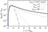Fig. 1 Normalized spectral electron fluxes downstream of the solar-wind termination shock according to Eq. (12). We show the kappa-distributed fluxes for different values of κ2,e. The special case κ2,e = 1.517 is our result for the perpendicular solar-wind termination shock according to Eq. (10).

3. Electric equilibrium potential

In the following, we calculate the electric equilibrium potential Φ up to which a spacecraft charges up when entering the heliosheath under the assumption that both electrons and protons have kappa-distributions and that emission processes are negligible in the plasma. Fahr & Siewert (2013) show that all ions (solar-wind as well as pick-up ions) treated as one fluid can be characterized as one joint kappa-function with a joint kappa-index κ_2,i ≃ 2, depending on the pick-up ion abundance downstream of the shock (see Fig. 2 of Fahr & Siewert 2013). Therefore, we describe electrons with Eq. (11) and protons with the following distribution downstream of the shock: ${\mathit{f}}_{\mathrm{2}\mathit{,}\mathrm{i}}\mathrm{\left(}\mathit{v}\mathrm{\right)}\mathrm{=}\frac{{\mathit{n}}_{\mathrm{2}\mathit{,}\mathrm{i}}}{{\mathit{\pi }}^{\mathrm{3}\mathit{/}\mathrm{2}}{\mathit{\kappa }}_{\mathrm{2}\mathit{,}\mathrm{i}}^{\mathrm{3}\mathit{/}\mathrm{2}}{\mathrm{\Theta }}_{\mathrm{2}\mathit{,}\mathrm{i}}^{\mathrm{3}}}\frac{\mathrm{\Gamma }\mathrm{(}{\mathit{\kappa }}_{\mathrm{2}\mathit{,}\mathrm{i}}\mathrm{+}\mathrm{1}\mathrm{)}}{\mathrm{\Gamma }\mathrm{(}{\mathit{\kappa }}_{\mathrm{2}\mathit{,}\mathrm{i}}\mathrm{-}\mathrm{1}\mathit{/}\mathrm{2}\mathrm{)}}{\left[\mathrm{1}\mathrm{+}\frac{{\mathit{v}}^{\mathrm{2}}}{{\mathit{\kappa }}_{\mathrm{2}\mathit{,}\mathrm{i}}{\mathrm{\Theta }}_{\mathrm{2}\mathit{,}\mathrm{i}}^{\mathrm{2}}}\right]}^{\mathrm{-}\mathrm{(}{\mathit{\kappa }}_{\mathrm{2}\mathit{,}\mathrm{i}}\mathrm{+}\mathrm{1}\mathrm{)}}\mathrm{·}$(13)We assume that quasineutrality prevails outside of perturbed Debye regions, i.e., n_2,e = n_2,i.

Any metallic body embodied in the heliosheath plasma downstream of the shock charges up to an electric equilibrium potential Φ₂, which guarantees equal fluxes of ions and electrons reaching the metallic surface of this body per unit time (geometry taken to be planar). This behavior leads to the following requirement (after dropping downstream indices “2” for simplification): 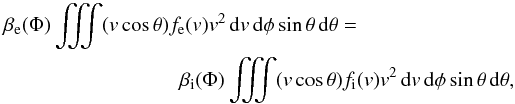$\begin{array}{ccc}{\mathit{\beta }}_{\mathrm{e}}\mathrm{\left(}\mathrm{\Phi }\mathrm{\right)}\$\mathrm{\left(}\mathit{v}\cos \mathit{\theta }\mathrm{\right)}{\mathit{f}}_{\mathrm{e}}\mathrm{\left(}\mathit{v}\mathrm{\right)}{\mathit{v}}^{\mathrm{2}}\hspace{0.17em}\mathrm{d}\mathit{v}\hspace{0.17em}\mathrm{d}\mathit{\phi }\sin \mathit{\theta }\hspace{0.17em}\mathrm{d}\mathit{\theta }\mathrm{=}& & \\ {\mathit{\beta }}_{\mathrm{i}}\mathrm{\left(}\mathrm{\Phi }\mathrm{\right)}\$\mathrm{\left(}\mathit{v}\cos \mathit{\theta }\mathrm{\right)}{\mathit{f}}_{\mathrm{i}}\mathrm{\left(}\mathit{v}\mathrm{\right)}{\mathit{v}}^{\mathrm{2}}\hspace{0.17em}\mathrm{d}\mathit{v}\hspace{0.17em}\mathrm{d}\mathit{\phi }\sin \mathit{\theta }\hspace{0.17em}\mathrm{d}\mathit{\theta ,}& & \end{array}$(14)where β_e(Φ) and β_i(Φ) denote the Boltzmann screening factors for electrons and ions, respectively. These factors describe the fraction of particles that can reach the wall against the electric potential Φ. The assumption of isotropic distribution functions leads to 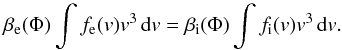${\mathit{\beta }}_{\mathrm{e}}\mathrm{\left(}\mathrm{\Phi }\mathrm{\right)}\mathrm{\int }{\mathit{f}}_{\mathrm{e}}\mathrm{\left(}\mathit{v}\mathrm{\right)}{\mathit{v}}^{\mathrm{3}}\hspace{0.17em}\mathrm{d}\mathit{v}\mathrm{=}{\mathit{\beta }}_{\mathrm{i}}\mathrm{\left(}\mathrm{\Phi }\mathrm{\right)}\mathrm{\int }{\mathit{f}}_{\mathrm{i}}\mathrm{\left(}\mathit{v}\mathrm{\right)}{\mathit{v}}^{\mathrm{3}}\hspace{0.17em}\mathrm{d}\mathit{v}\mathit{.}$(15)We expect that the resulting equilibrium potential Φ only affects the lowest-energy part of the distribution functions. Therefore, the Gaussian core of the kappa-distributed particles is the only screened population, leading to 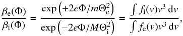$\frac{{\mathit{\beta }}_{\mathrm{e}}\mathrm{\left(}\mathrm{\Phi }\mathrm{\right)}}{{\mathit{\beta }}_{\mathrm{i}}\mathrm{\left(}\mathrm{\Phi }\mathrm{\right)}}\mathrm{=}\frac{\exp \mathrm{(}\mathrm{+}\mathrm{2}\mathit{e}\mathrm{\Phi }\mathit{/}\mathit{m}{{\mathrm{\Theta }}_{\mathrm{e}}^{\mathrm{2}}}^{\mathrm{)}}}{\exp \mathrm{(}\mathrm{-}\mathrm{2}\mathit{e}\mathrm{\Phi }\mathit{/}\mathit{M}{{\mathrm{\Theta }}_{\mathrm{i}}^{\mathrm{2}}}^{\mathrm{)}}}\mathrm{=}\frac{\mathrm{\int }{\mathit{f}}_{\mathrm{i}}\mathrm{\left(}\mathit{v}\mathrm{\right)}{\mathit{v}}^{\mathrm{3}}\hspace{0.17em}\mathrm{d}\mathit{v}}{\mathrm{\int }{\mathit{f}}_{\mathrm{e}}\mathrm{\left(}\mathit{v}\mathrm{\right)}{\mathit{v}}^{\mathrm{3}}\hspace{0.17em}\mathrm{d}\mathit{v}}\mathit{,}$(16)which can be rewritten as $\exp \left[\mathrm{2}\mathit{e}\mathrm{\Phi }\left(\frac{\mathrm{1}}{\mathit{m}{\mathrm{\Theta }}_{\mathrm{e}}^{\mathrm{2}}}\mathrm{+}\frac{\mathrm{1}}{\mathit{M}{\mathrm{\Theta }}_{\mathrm{i}}^{\mathrm{2}}}\right)\right]\mathrm{=}\frac{\mathrm{\int }{\mathit{f}}_{\mathrm{i}}\mathrm{\left(}\mathit{v}\mathrm{\right)}{\mathit{v}}^{\mathrm{3}}\hspace{0.17em}\mathrm{d}\mathit{v}}{\mathrm{\int }{\mathit{f}}_{\mathrm{e}}\mathrm{\left(}\mathit{v}\mathrm{\right)}{\mathit{v}}^{\mathrm{3}}\hspace{0.17em}\mathrm{d}\mathit{v}}\mathrm{·}$(17)We solve the remaining integrals in the above expression with Θ_2,i/ Θ_2,e ≈ m/M, leading to $\frac{\mathrm{\int }{\mathit{f}}_{\mathrm{i}}\mathrm{\left(}\mathit{v}\mathrm{\right)}{\mathit{v}}^{\mathrm{3}}\hspace{0.17em}\mathrm{d}\mathit{v}}{\mathrm{\int }{\mathit{f}}_{\mathrm{e}}\mathrm{\left(}\mathit{v}\mathrm{\right)}{\mathit{v}}^{\mathrm{3}}\hspace{0.17em}\mathrm{d}\mathit{v}}\mathrm{=}\frac{\mathrm{\Gamma }\mathrm{(}{\mathit{\kappa }}_{\mathrm{i}}\mathrm{+}\mathrm{1}\mathrm{)}}{\mathrm{\Gamma }\mathrm{(}{\mathit{\kappa }}_{\mathrm{i}}\mathrm{-}\mathrm{1}\mathit{/}\mathrm{2}\mathrm{)}}\frac{\mathrm{\Gamma }\mathrm{(}{\mathit{\kappa }}_{\mathrm{e}}\mathrm{-}\mathrm{1}\mathit{/}\mathrm{2}\mathrm{)}}{\mathrm{\Gamma }\mathrm{(}{\mathit{\kappa }}_{\mathrm{e}}\mathrm{+}\mathrm{1}\mathrm{)}}\frac{\sqrt{{\mathit{\kappa }}_{\mathrm{e}}\mathit{m}}\mathrm{(}{\mathit{\kappa }}_{\mathrm{e}}\mathrm{-}{\mathrm{1}}^{\mathrm{)}}}{\sqrt{{\mathit{\kappa }}_{\mathrm{i}}\mathit{M}}\mathrm{(}{\mathit{\kappa }}_{\mathrm{i}}\mathrm{-}{\mathrm{1}}^{\mathrm{)}}}\mathrm{·}$(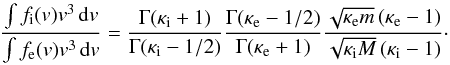18)We find (with $\mathrm{\Pi }\mathrm{=}{\mathrm{\Theta }}_{\mathrm{2}\mathit{,}\mathrm{e}}^{\mathrm{2}}\mathit{/}{\mathrm{\Theta }}_{\mathrm{1}\mathit{,}\mathrm{e}}^{\mathrm{2}}\mathrm{\approx }\mathrm{1}$) $\exp \left[\frac{\mathrm{2}\mathit{e}\mathrm{\Phi }}{\mathit{m}{\mathit{U}}_{\mathrm{1}}^{\mathrm{2}}}\left(\frac{{\mathit{U}}_{\mathrm{1}}^{\mathrm{2}}}{{\mathrm{\Theta }}_{\mathrm{e}}^{\mathrm{2}}}\mathrm{+}\frac{\mathit{m}{\mathit{U}}_{\mathrm{1}}^{\mathrm{2}}}{\mathit{M}{\mathrm{\Theta }}_{\mathrm{i}}^{\mathrm{2}}}\right)\right]\mathrm{=}\exp \left[\frac{\mathrm{2}\mathit{e}\mathrm{\Phi }}{\mathit{M}{\mathit{U}}_{\mathrm{1}}^{\mathrm{2}}}\mathrm{(}{\mathit{\mu }}_{\mathrm{1}\mathit{,}\mathrm{e}}^{\mathrm{2}}\mathrm{+}{{\mathit{\mu }}_{\mathrm{1}\mathit{,}\mathrm{i}}^{\mathrm{\ast }\mathrm{2}}}^{\mathrm{)}}\right]\mathit{,}$(19)where μ_1,e and ${\mathit{\mu }}_{\mathrm{1}\mathit{,}\mathrm{i}}^{\mathrm{\ast }}$ denote the upstream solar-wind electron and pick-up ion Mach numbers. These numbers are given by values of the order μ_1,e ≃ 10 and ${\mathit{\mu }}_{\mathrm{1}\mathit{,}\mathrm{i}}^{\mathrm{\ast }}\mathrm{\simeq }\mathrm{3}$. Therefore, 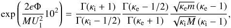$\exp \left(\frac{\mathrm{2}\mathit{e}\mathrm{\Phi }}{\mathit{M}{\mathit{U}}_{\mathrm{1}}^{\mathrm{2}}}{\mathrm{10}}^{\mathrm{2}}\right)\mathrm{=}\frac{\mathrm{\Gamma }\mathrm{(}{\mathit{\kappa }}_{\mathrm{i}}\mathrm{+}\mathrm{1}\mathrm{)}}{\mathrm{\Gamma }\mathrm{(}{\mathit{\kappa }}_{\mathrm{i}}\mathrm{-}\mathrm{1}\mathit{/}\mathrm{2}\mathrm{)}}\frac{\mathrm{\Gamma }\mathrm{(}{\mathit{\kappa }}_{\mathrm{e}}\mathrm{-}\mathrm{1}\mathit{/}\mathrm{2}\mathrm{)}}{\mathrm{\Gamma }\mathrm{(}{\mathit{\kappa }}_{\mathrm{e}}\mathrm{+}\mathrm{1}\mathrm{)}}\frac{\sqrt{{\mathit{\kappa }}_{\mathrm{e}}\mathit{m}}\mathrm{(}{\mathit{\kappa }}_{\mathrm{e}}\mathrm{-}{\mathrm{1}}^{\mathrm{)}}}{\sqrt{{\mathit{\kappa }}_{\mathrm{i}}\mathit{M}}\mathrm{(}{\mathit{\kappa }}_{\mathrm{i}}\mathrm{-}{\mathrm{1}}^{\mathrm{)}}}\mathit{,}$(20)which leads to the following potential $\mathrm{\Phi }\mathrm{=}\frac{\mathit{M}{\mathit{U}}_{\mathrm{1}}^{\mathrm{2}}}{\mathrm{200}\mathit{e}}\ln \left[\frac{\mathrm{\Gamma }\mathrm{(}{\mathit{\kappa }}_{\mathrm{i}}\mathrm{+}\mathrm{1}\mathrm{)}}{\mathrm{\Gamma }\mathrm{(}{\mathit{\kappa }}_{\mathrm{i}}\mathrm{-}\mathrm{1}\mathit{/}\mathrm{2}\mathrm{)}}\frac{\mathrm{\Gamma }\mathrm{(}{\mathit{\kappa }}_{\mathrm{e}}\mathrm{-}\mathrm{1}\mathit{/}\mathrm{2}\mathrm{)}}{\mathrm{\Gamma }\mathrm{(}{\mathit{\kappa }}_{\mathrm{e}}\mathrm{+}\mathrm{1}\mathrm{)}}\frac{\sqrt{{\mathit{\kappa }}_{\mathrm{e}}\mathit{m}}\mathrm{(}{\mathit{\kappa }}_{\mathrm{e}}\mathrm{-}{\mathrm{1}}^{\mathrm{)}}}{\sqrt{{\mathit{\kappa }}_{\mathrm{i}}\mathit{M}}\mathrm{(}{\mathit{\kappa }}_{\mathrm{i}}\mathrm{-}{\mathrm{1}}^{\mathrm{)}}}\right]\mathrm{·}$(21)As a consistency check, we note that this expression leads to the classical plasma-physics formula for Φ = Φ_c in the limit of Maxwellian distributions (i.e., κ_e = κ_i → ∞) with identical temperatures ${\mathit{T}}_{\mathrm{i}}\mathrm{=}{\mathit{T}}_{\mathrm{e}}\mathrm{=}\mathit{M}{\mathit{U}}_{\mathrm{1}}^{\mathrm{2}}\mathit{/}\mathrm{200}$ K.

In Fig. 2, we show the resulting electric potential Φ as a function of the prevailing kappa-index κ_2,e of the shock-heated downstream electrons. This profile shows that the expected equilibrium potential drops to values of Φ ≤ −30 V in the range of expected indices 1.5 ≤ κ_e ≤ 2. This potential does not allow electrons with energies below 30 eV to reach the detector.

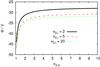Fig. 2 Equilibrium potential of a metallic body in the presence of kappa-distributed ions and electrons according to Eq. (21). We show the potential as a function of κ2,e for different values of κ2,i. We assume U1 = 400 km s-1.

4. Degenerated Debye length

The degeneration of the Debye length is a direct consequence of highly nonthermal kappa-type distribution functions. The electric screening by plasma-electron distributions with a largely extended power-law tail is significantly less efficient compared to the screening by Maxwellian thermal electrons with temperature T_e. Maxwellian thermal electrons lead to the classical Debye-screening length of 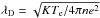${\mathit{\lambda }}_{\mathrm{D}}\mathrm{=}\sqrt{\mathit{K}{\mathit{T}}_{\mathrm{e}}\mathit{/}\mathrm{4}\mathit{\pi n}{\mathit{e}}^{\mathrm{2}}}$. The effect of degenerating Debye lengths has been recognized and emphasized by Treumann et al. (2004), finding that the resulting Debye length ${\mathit{\lambda }}_{\mathrm{D}}^{\mathit{\kappa }}$ may easily increase by factors of ${\mathit{\lambda }}_{\mathrm{D}}^{\mathit{\kappa }}\mathit{/}{\mathit{\lambda }}_{\mathrm{D}}\mathrm{\ge }{\mathrm{10}}^{\mathrm{6}}$ for low electron kappa-indices of κ_e ≃ 1.5. With a more relaxed approach, yet along the lines of these authors’ discussion, we obtain the following very similar conclusions.

For the description of the effective screening of kappa electrons, we simply replace the Maxwellian temperature T_e by the corresponding electron kappa temperature ${\mathit{T}}_{\mathrm{e}}^{\mathit{\kappa }}$, which is given by$\mathit{K}{\mathit{T}}_{\mathrm{e}}^{\mathit{\kappa }}\mathrm{=}\frac{{\mathit{P}}_{\mathrm{e}}^{\mathit{\kappa }}}{{\mathit{n}}_{\mathrm{e}}}\mathrm{=}\frac{\mathit{m}}{\mathrm{2}}{\mathrm{\Theta }}_{\mathrm{e}}^{\mathrm{2}}\frac{{\mathit{\kappa }}_{\mathrm{e}}}{{\mathit{\kappa }}_{\mathrm{e}}\mathrm{-}\mathrm{3}\mathit{/}\mathrm{2}}\mathrm{·}$(22)Consequently, we find ${\mathit{\lambda }}_{\mathrm{D}}^{\mathit{\kappa }}\mathit{/}{\mathit{\lambda }}_{\mathrm{D}}\mathrm{=}\sqrt{{\mathit{T}}_{\mathrm{e}}^{\mathit{\kappa }}\mathit{/}{\mathit{T}}_{\mathrm{e}}}\mathrm{=}\sqrt{\frac{\mathit{m}}{\mathrm{2}}{\mathrm{\Theta }}_{\mathrm{e}}^{\mathrm{2}}\frac{{\mathit{\kappa }}_{\mathrm{e}}}{{\mathit{\kappa }}_{\mathrm{e}}\mathrm{-}\mathrm{3}\mathit{/}\mathrm{2}}\mathit{/}\mathit{K}{\mathit{T}}_{\mathrm{e}}}\mathit{.}$(23)Assuming that the core of the kappa distribution is identical to the Maxwellian core (i.e., $\mathit{m}{\mathrm{\Theta }}_{\mathrm{e}}^{\mathrm{2}}\mathrm{=}\mathrm{2}\mathit{K}{\mathit{T}}_{\mathrm{e}}$), we obtain the following result for the effective Debye length: ${\mathit{\lambda }}_{\mathrm{D}}^{\mathit{\kappa }}\mathrm{=}{\mathit{\lambda }}_{\mathrm{D}}\sqrt{\frac{{\mathit{\kappa }}_{\mathrm{e}}}{{\mathit{\kappa }}_{\mathrm{e}}\mathrm{-}\mathrm{3}\mathit{/}\mathrm{2}}}\mathrm{·}$(24)This modified Debye length has an interesting effect on the propagation of plasma waves. The general dispersion relation for electron-acoustic plasma waves (e.g., see Chen 1974, Eqs. (4)–(48)) is given by $\frac{\mathit{\omega }}{\mathit{k}}\mathrm{=}\sqrt{\frac{\mathit{K}{\mathit{T}}_{\mathrm{e}}^{\mathit{\kappa }}}{\mathit{M}}\frac{\mathrm{1}}{\mathrm{1}\mathrm{+}{\mathrm{(}\mathit{k}{{\mathit{\lambda }}_{\mathrm{D}}^{\mathit{\kappa }}}^{\mathrm{)}}}^{\mathrm{2}}}\mathrm{+}\frac{\mathit{K}{\mathit{T}}_{\mathrm{i}}}{\mathit{M}}}\mathrm{·}$(25)In the general case of ${\mathit{T}}_{\mathrm{e}}^{\mathit{\kappa }}\mathrm{\gg }{\mathit{T}}_{\mathit{i}}$, and for very small wavevector values of $\mathit{k}\mathrm{\equiv }\mathrm{2}\mathit{\pi }\mathit{/}\mathit{\lambda }\mathrm{\ll }\mathrm{2}\mathit{\pi }\mathit{/}{\mathit{\lambda }}_{\mathrm{D}}^{\mathit{\kappa }}$, this dispersion relation allows for a branch of electron-acoustic waves that propagate with a phase/group velocity of $\frac{\mathit{\omega }}{\mathit{k}}\mathrm{=}\frac{\mathit{\partial \omega }}{\mathit{\partial k}}\mathrm{=}\sqrt{\frac{\mathit{K}{\mathit{T}}_{\mathrm{e}}^{\mathit{\kappa }}}{\mathit{M}}}\mathrm{=}\sqrt{\frac{\mathit{m}}{\mathrm{2}\mathit{M}}{\mathrm{\Theta }}_{\mathrm{e}}^{\mathrm{2}}\frac{{\mathit{\kappa }}_{\mathrm{e}}}{{\mathit{\kappa }}_{\mathrm{e}}\mathrm{-}\mathrm{3}\mathit{/}\mathrm{2}}}\mathrm{·}$(26)This branch is a special kappa-mode propagating with a typical phase or group velocity that directly depends on the electron kappa index κ_e. Testing plasma acoustic waves in this range of large wavelengths should hence directly reveal the prevailing kappa index κ_e and, therefore, the character of the suprathermal downstream electrons.

On the other hand, the limit of larger wavevectors with $\mathit{k}\mathrm{\equiv }\mathrm{2}\mathit{\pi }\mathit{/}\mathit{\lambda }\mathrm{\ge }\mathrm{2}\mathit{\pi }\mathit{/}{\mathit{\lambda }}_{\mathrm{D}}^{\mathit{\kappa }}$ allows for a branch of nonpropagating waves (i.e., standing oscillations) with plasma eigenfrequencies given by $\frac{\mathit{\omega }}{\mathit{k}}\mathrm{=}\sqrt{\frac{\mathit{K}{\mathit{T}}_{\mathrm{e}}^{\mathit{\kappa }}}{\mathit{M}}\frac{\mathrm{1}}{{\mathrm{(}\mathit{k}{{\mathit{\lambda }}_{\mathrm{D}}^{\mathit{\kappa }}}^{\mathrm{)}}}^{\mathrm{2}}}}\mathrm{·}$(27)With Eqs. (22) and (24), we can write $\mathit{\omega }\mathrm{=}\sqrt{\frac{\mathit{K}{\mathit{T}}_{\mathrm{e}}^{\mathit{\kappa }}}{\mathit{M}{\mathit{\lambda }}_{\mathrm{D}}^{\mathit{\kappa }\mathrm{2}}}}\mathrm{=}\sqrt{\frac{\frac{\mathit{m}}{\mathrm{2}}{\mathrm{\Theta }}_{\mathrm{e}}^{\mathrm{2}}\frac{{\mathit{\kappa }}_{\mathrm{e}}}{{\mathit{\kappa }}_{\mathrm{e}}\mathrm{-}\mathrm{3}\mathit{/}\mathrm{2}}}{\mathit{M}{\mathit{\lambda }}_{\mathrm{D}}^{\mathrm{2}}\mathrm{(}{\frac{{\mathit{\kappa }}_{\mathrm{e}}}{{\mathit{\kappa }}_{\mathrm{e}}\mathrm{-}\mathrm{3}\mathit{/}\mathrm{2}}}^{\mathrm{)}}}}\mathrm{=}\sqrt{\frac{\mathrm{4}\mathit{\pi n}{\mathit{e}}^{\mathrm{2}}}{\mathit{M}}}\mathrm{=}\mathit{\omega }p$(28)for these oscillations. Under these conditions, the plasma, surprisingly enough, does not oscillate with the electron plasma frequency ω_e, but it does oscillate with the ion plasma frequency ω_p, which is a phenomenon that only quite rarely occurs in nature. The plasma oscillations recently registered by Voyager-1 (Gurnett et al. 2013), which were interpreted as electron plasma oscillations, may perhaps be reinterpreted as this type of ion plasma oscillations. As such, they would allow us to infer environmental plasma densities of the order n ≃ (m/M)0.1 cm^-3 ≤ 10^-4 cm^-3.

5. Calculation of Π in view of the downstream electron instabilities

In Sect. 2, we introduced the quantity Π (see Eq. (4)), which denotes the ratio of the thermal core widths, $\mathrm{\Pi }\mathrm{=}{\mathrm{\Theta }}_{\mathrm{2}\mathit{,}\mathrm{e}}^{\mathrm{2}}\mathit{/}{\mathrm{\Theta }}_{\mathrm{1}\mathit{,}\mathrm{e}}^{\mathrm{2}}$. Until this point, we did not determine a reasonable value for Π. Previous expressions based on an upstream-downstream transformation of thermal-core velocities (Fahr & Siewert 2013) appear to be irrelevant since their calculation relies on the assumption that upstream core electrons are independently transformed simply into downstream core electrons according to the Liouville-Vlasov theorem. In reality, however, all upstream electrons overshoot to the downstream side where the action of instabilities, such as the two-stream instability or the Buneman instability, redistribute and isotropize them. In the case of the two-stream instability (e.g., see Chen 1974), electrons can excite ion oscillations as long as their velocities are greater than the thermal core velocities of the protons. This fast relaxation of the electron distribution function toward the downstream ion distribution function then leads to a quasiequilibrium distribution.

Consistent forms of such quasi-equilibria between particle distribution functions and turbulence power spectra have been investigated in Sect. 2.5 in Fahr & Fichtner (2011) and, for steady state conditions, by Yoon (2011, 2012) and Zaheer & Yoon (2013). In all of these cases, the asymptotic state results in kappa distributions. Also, in our case, as a result of a shock-induced electron injection with velocity-space diffusion and relaxation described by a phase-space transport equation of the type $\frac{\mathit{\partial }{\mathit{f}}_{\mathrm{e}}}{\mathit{\partial t}}\mathrm{=}\frac{\mathrm{1}}{{\mathit{v}}^{\mathrm{2}}}\frac{\mathit{\partial }}{\mathit{\partial v}}\left({\mathit{v}}^{\mathrm{2}}{\mathit{D}}_{\mathit{vv}}\frac{\mathit{\partial }{\mathit{f}}_{\mathrm{e}}}{\mathit{\partial v}}\right)\mathrm{+}\frac{{\mathit{f}}_{\mathrm{e}}\mathrm{-}{\mathit{f}}_{\mathrm{p}}}{{\mathit{\tau }}_{\mathrm{ep}}}\mathit{,}$(29)we expect solutions in form of kappa distributions. In fact, as shown by Treumann et al. (2004), this kind of transport equations leads to a quasi-equilibrium distribution in the form of a kappa distribution with a thermal core given by the downstream ion velocities: ${\mathrm{\Theta }}_{\mathrm{2}\mathit{,}\mathrm{e}}^{\mathrm{2}}\mathrm{\left(}{\mathit{f}}_{\mathrm{p}}\mathrm{\right)}\mathrm{\simeq }\mathrm{2}{\mathit{P}}_{\mathrm{2}\mathit{,}\mathrm{p}}\mathit{/}{\mathit{n}}_{\mathrm{2}\mathit{,}\mathrm{e}}\mathit{m}$. We finally find (using Eq. (4) in Fahr & Siewert 2013) $\mathrm{\Pi }\mathrm{=}{\mathrm{\Theta }}_{\mathrm{2}\mathit{,}\mathrm{e}}^{\mathrm{2}}\mathit{/}{\mathrm{\Theta }}_{\mathrm{1}\mathit{,}\mathrm{e}}^{\mathrm{2}}\mathrm{=}\frac{\mathrm{2}{\mathit{P}}_{\mathrm{2}\mathit{,}\mathrm{p}}{\mathit{n}}_{\mathrm{1}}\mathit{m}}{\mathrm{3}{\mathit{P}}_{\mathrm{1}\mathit{,}\mathrm{p}}{\mathit{n}}_{\mathrm{2}\mathit{,}\mathrm{e}}\mathit{m}}\mathrm{=}\frac{\mathrm{2}}{\mathrm{9}}\left[\mathrm{2}\mathit{A}\mathrm{\left(}\mathit{s,\alpha }\mathrm{\right)}\mathrm{+}\mathit{B}\mathrm{\left(}\mathit{s,\alpha }\mathrm{\right)}\right]$(30)with $\mathit{A}\mathrm{\left(}\mathit{s,\alpha }\mathrm{\right)}\mathrm{=}\sqrt{{\cos }^{\mathrm{2}}\mathit{\alpha }\mathrm{+}{\mathit{s}}^{\mathrm{2}}{\sin }^{\mathrm{2}}\mathit{\alpha }}$ and B(s,α) = s²/A²(s,α).

The above expression for a perpendicular shock with s = 2.5 (Richardson et al. 2008) leads to Π(α = π/ 2) = 1.33. This finally shows that the quantity Π is, in fact, of order unity, verifying a posteriori all of our above results that we calculated for Π = 1. Using this more precise value for Π, Eq. (10) leads to a marginally different value for the kappa-index of κ_2,e = 1.522.

6. Summary and conclusions

Previous studies suggest that strongly-heated solar-wind electrons should appear in measurements as accelerated suprathermal particles downstream of the termination shock. However, these electrons were not observed by Voyager in the heliosheath. We investigate this apparent contradiction and find that heliosheath electrons are distributed according to a kappa-type distribution function with an extended suprathermal tail (see Fig. 1). These highly suprathermal kappa-distributed electrons lead to a

strong negative charging of all metallic bodies exposed to this plasma environment, consequently also charging up the Voyager spacecraft.

A spacecraft potential of the order −30 V, as calculated in Fig. 2, has a significant effect on the Voyager electron measurements in the heliosheath. Under these conditions, it repels thermal electrons in the energy range below 30 eV, leading to an increase in the previously determined upper limit of 3 eV (Richardson et al. 2008) for the electron temperature. The ions, on the other hand, are accelerated into the Faraday cups. The difference in the derived bulk speeds, however, is negligible: corrected for a −30 V potential, the radial downstream proton bulk velocity increases from 130 km s^-1 to about 132 km s^-1.

In addition, this suprathermal distribution of downstream electrons also results in an unusually enlarged Debye length. As a consequence of this effect, the phase velocity v_φ = ω/k of electrostatic plasma waves depends on the effective kappa temperature of the electrons in the heliosheath plasma environment. The detection of these plasma waves allows us to infer the effective kappa electron temperature as an observable quantity. These distributions also permit a type of nonpropagating standing waves with the ion plasma frequency ω_p as their eigen frequency.

References

All Figures

	Fig. 1 Normalized spectral electron fluxes downstream of the solar-wind termination shock according to Eq. (12). We show the kappa-distributed fluxes for different values of κ2,e. The special case κ2,e = 1.517 is our result for the perpendicular solar-wind termination shock according to Eq. (10).
In the text

	Fig. 2 Equilibrium potential of a metallic body in the presence of kappa-distributed ions and electrons according to Eq. (21). We show the potential as a function of κ2,e for different values of κ2,i. We assume U1 = 400 km s-1.
In the text

References

- Baumjohann, W., & Treumann, R. A. 1996, Basic space plasma physics (London: Imperial College Press) [Google Scholar]
- Chalov, S. V., & Fahr, H. J. 2013, MNRAS, 433, L40 [NASA ADS] [Google Scholar]
- Chashei, I. V., & Fahr, H. J. 2013, Annales Geophysicae, 31, 1205 [Google Scholar]
- Chashei, I. V., & Fahr, H. J. 2014, Sol. Phys., 289, 1359 [NASA ADS] [CrossRef] [Google Scholar]
- Chen, F. F. 1974, Introduction to plasma physics (New York: Plenum Press) [Google Scholar]
- Decker, R. B., Krimigis, S. M., Roelof, E. C., et al. 2008, Nature, 454, 67 [NASA ADS] [CrossRef] [PubMed] [Google Scholar]
- Diver, D. A. 2001, A plasma formulary for physics, technology, and astrophysics (Berlin: Wiley-VcH) [Google Scholar]
- Erkaev, N. V., Vogl, D. F., & Biernat, H. K. 2000, J. Plasma Physics, 64, 561 [Google Scholar]
- Fahr, H. J., & Fichtner, H. 2011, A&A, 533, A92 [NASA ADS] [CrossRef] [EDP Sciences] [Google Scholar]
- Fahr, H.-J., & Siewert, M. 2007, Astrophys. Space Sci. Trans., 3, 21 [Google Scholar]
- Fahr, H.-J., & Siewert, M. 2010, A&A, 512, A64 [NASA ADS] [CrossRef] [EDP Sciences] [Google Scholar]
- Fahr, H.-J., & Siewert, M. 2011, A&A, 527, A125 [NASA ADS] [CrossRef] [EDP Sciences] [Google Scholar]
- Fahr, H.-J., & Siewert, M. 2013, A&A, 558, A41 [NASA ADS] [CrossRef] [EDP Sciences] [Google Scholar]
- Fahr, H.-J., & Siewert, M. 2015, A&A, 576, A100 [NASA ADS] [CrossRef] [EDP Sciences] [Google Scholar]
- Fahr, H.-J., Siewert, M., & Chashei, I. 2012, Ap&SS, 341, 265 [Google Scholar]
- Fahr, H. J., Chashei, I. V., & Verscharen, D. 2014, A&A, 571, A78 [NASA ADS] [CrossRef] [EDP Sciences] [Google Scholar]
- Gombosi, T. I. 1998, Physics of the space environment (New York: Cambridge University Press) [Google Scholar]
- Goodrich, C. C., & Scudder, J. D. 1984, J. Geophys. Res., 89, 6654 [NASA ADS] [CrossRef] [Google Scholar]
- Gurnett, D. A., Kurth, W. S., Burlaga, L. F., & Ness, N. F. 2013, AGU Fall Meeting Abstracts, B1 [Google Scholar]
- Heerikhuisen, J., Pogorelov, N. V., Florinski, V., Zank, G. P., & le Roux, J. A. 2008, ApJ, 682, 679 [NASA ADS] [CrossRef] [Google Scholar]
- Hudson, P. D. 1970, Planet. Space Sci., 18, 1611 [NASA ADS] [CrossRef] [Google Scholar]
- Lembège, B., Savoini, P., Balikhin, M., Walker, S., & Krasnoselskikh, V. 2003, J. Geophys. Res., 108, 1256 [CrossRef] [Google Scholar]
- Lembège, B., Giacalone, J., Scholer, M., et al. 2004, Space Sci. Rev., 110, 161 [NASA ADS] [CrossRef] [Google Scholar]
- Leroy, M. M., & Mangeney, A. 1984, Annales Geophysicae, 2, 449 [Google Scholar]
- Leroy, M. M., Winske, D., Goodrich, C. C., Wu, C. S., & Papadopoulos, K. 1982, J. Geophys. Res., 87, 5081 [NASA ADS] [CrossRef] [Google Scholar]
- Richardson, J. D., Kasper, J. C., Wang, C., Belcher, J. W., & Lazarus, A. J. 2008, Nature, 454, 63 [NASA ADS] [CrossRef] [PubMed] [Google Scholar]
- Schwartz, S. J., Thomsen, M. F., Bame, S. J., & Stansberry, J. 1988, J. Geophys. Res., 93, 12923 [NASA ADS] [CrossRef] [Google Scholar]
- Serrin, J. 1959, Handbuch der Physik, 8, 125 [NASA ADS] [CrossRef] [Google Scholar]
- Tokar, R. L., Aldrich, C. H., Forslund, D. W., & Quest, K. B. 1986, Phys. Rev. Lett., 56, 1059 [NASA ADS] [CrossRef] [Google Scholar]
- Treumann, R. A., Jaroschek, C. H., & Scholer, M. 2004, Phys. Plasmas, 11, 1317 [NASA ADS] [CrossRef] [Google Scholar]
- Yoon, P. H. 2011, Phys. Plasmas, 18, 122303 [Google Scholar]
- Yoon, P. H. 2012, Phys. Plasmas, 19, 012304 [NASA ADS] [CrossRef] [Google Scholar]
- Zaheer, S., & Yoon, P. H. 2013, ApJ, 775, 108 [NASA ADS] [CrossRef] [Google Scholar]
- Zank, G. P., Heerikhuisen, J., Pogorelov, N. V., Burrows, R., & McComas, D. 2010, ApJ, 708, 1092 [NASA ADS] [CrossRef] [Google Scholar]