| Issue |
A&A
Volume 579, July 2015
|
|
|---|---|---|
| Article Number | L9 | |
| Number of page(s) | 5 | |
| Section | Letters | |
| DOI | https://doi.org/10.1051/0004-6361/201525668 | |
| Published online | 15 July 2015 | |
Search for signatures of dust in the Pluto–Charon system using Herschel/PACS observations⋆,⋆⋆
1
Konkoly Observatory, Research Centre for Astronomy and Earth Sciences,
Hungarian Academy of Sciences, Konkoly Thege Miklós út 15-17, 1121
Budapest, Hungary
e-mail: This email address is being protected from spambots. You need JavaScript enabled to view it.
2
Max-Planck-Institut für Astronomie, Königstuhl 17, 69117
Heidelberg,
Germany
3
Observatoire de Paris, CNRS, UPMC Univ. Paris 06,
Univ. Paris-Diderot, 5 place Jules
Janssen, 92195
Meudon Principal Cedex,
France
Received:
15
January
2015
Accepted:
25
June
2015
Abstract
In this letter we explore the environment of Pluto and Charon in the far infrared with the main aim of identifying the signs of any possible dust ring, should it exist in the system. Our study is based on observations performed at 70 μm with the PACS instrument onboard the Herschel Space Observatory at nine epochs between March 14 and 19, 2012. The far-infrared images of the Pluto–Charon system are compared to those of the point spread function (PSF) reference quasar 3C 454.3. The deviation between the observed Pluto–Charon and reference PSFs are less then 1σ, indicating that clear evidence for an extended dust ring around the system was not found. Our method is capable of detecting a hypothetical ring with a total flux of ~3.3 mJy at a distance of ~153 000 km (~8.2 Pluto–Charon distances) from the system’s barycentre. We place upper limits on the total disk mass and on the column density in a reasonable disk configuration and analyse the hazard during the flyby of NASA’s New Horizons in July 2015. This realistic model configuration predicts a column density of 8.7 × 10⁻¹⁰ g cm-2 along the path of the probe and an impactor mass of 8.7 × 10⁻⁵ g.
Key words: planets and satellites: rings / planets and satellites: individual: Pluto / planets and satellites: individual: Charon
Herschel is an ESA space observatory with science instruments provided by European-led Principal Investigator consortia and with important participation from NASA.
Appendices are available in electronic form at http://www.aanda.org
© ESO, 2015
1. Introduction
The Pluto–Charon system harbours at least four smaller satellites. Nix and Hydra (Weaver et al. 2006; Buie et al. 2006) have diameters estimated to be around 100 km or less, while Kerberos and Styx (Showalter et al. 2011, 2012) have diameters less than 40 km. Studies of the phase space (Nagy et al. 2006; Süli & Zsigmond 2009; Giuliatti et al. 2010, 2013; Zsigmond & Süli 2010; Pires et al. 2011) have shown that dynamically stable regions exist around the system. Formation of a debris disk as a result of the collision of small bodies has also been suggested (Durda & Stern 2000; Steffl et al. 2006).
The possible existence of such a ring was investigated by Steffl & Stern (2007), but observational evidence for this ring was not found. They placed a 3σ upper limit on the azimuthally averaged normal I/F of ring particles of 5.1 × 10⁷ at a distance of 42 000 km from the Pluto–Charon barycentre. Boissel et al. (2014) derive an upper limit of 15 000 for the number of bodies smaller than 0.3 km at distances smaller than 70 000 km from Pluto’s system barycentre. The impactor velocity of colliding bodies ranges from 10−100 m s-1 (Steffl & Stern 2007). Given that the escape velocities of Nix and Hydra are between 30 and 90 m s-1, any material ejected from these bodies can escape from the satellites but not from the system. (The Pluto and Charon escape velocities are ~1200 and ~500 m s-1, respectively.) Recently, a ring system around the centaurs Chariklo (Braga-Ribas et al. 2014) has been discovered, and several indicators show that probably (2060) Chiron (Ortiz et al. 2015) harbours a ring system, too. These suggest that dust rings around small bodies may be a common feature.
The existence of a dust ring around the system would also mean a hazard for NASA’s “New Horizons” probe (Stern 2008). The goal of the mission is to provide the first in situ exploration of the system, with a close fly-by in July 2015.
Visual wavelength-range reflected-light observations (Showalter et al. 2011, 2012) taken with the Hubble Space Telescope (HST) are, however, not ideal for detecting diffuse material in the Pluto–Charon system owing to the very high brightness of Pluto and Charon and a possibly low surface brightness of the hypothetical ring. In the thermal infrared, the contrast between the central object (star) and the surrounding material (debris disk) is higher than in the visual range, due to the very different spectral energy distributions (SEDs) of the two components. In the case of Pluto, the thermal infrared may still be beneficial in the case of dark grains in the hypothetical ring, such as the ones found in the Uranus system (albedo of ~6%, Karkoschka 2001).
In this Letter we investigate thermal emission (70 μm) images of the Pluto–Charon system, taken with the Photodetector Array Camera and Spectrometer (PACS, Poglitsch et al. 2010) of the Herschel Space Observatory (Pilbratt et al. 2010), in order to identify any extended emission, originating in sources other than Pluto and Charon themselves.
Diffuse dust structures like disks and rings modify the point spread function (PSF) of their parent sources, even if they cannot be fully resolved. Partially resolved features – if bright enough – cause a broadening of the PSF of the source. This kind of broadening has been used to detect partially resolved debris disks with the PACS photometer in many cases (see e.g. Moór et al. 2015). In the case of PACS, the 70 μm band has the highest spatial resolution (FWHM of 5 7), and also the SED of large grains peaks around this wavelength at the heliocentric distance of Pluto. In the case of smaller grains, the temperature is higher than Pluto’s, causing a shortward shift of the peak of the SED, again favouring the shortest wavelength PACS band to detect it. The ratio of the fluxes from a disk/ring and Pluto is expected to be the highest in this band as well. Therefore we only use the 70 μm band data in the following analysis.
2. Observations and data reduction
The PACS camera on-board the Herschel observed the Pluto–Charon system several times. We used the light-curve measurement of Lellouch et al. (proposal ID: OT2_elellouc_2, Lellouch et al. 2013; and in prep.) taken at 70/160 μm between March 14 and 19 in 2012. All measurements were made in scan-map mode with a scan speed of 20′′ s-1 and lasted for 286 s. Pluto–Charon was observed at a heliocentric distance of r = 32.2 au and at a distance of Δ≃ 32.4 au from the telescope. The basic characteristics of the Pluto observations are listed in Table A.1.
In addition to the target measurements, we used the engineering observations of the fiducial star α Boo for calibration purposes, as well as 42 Herschel/PACS measurements of the quasar 3C 454.3 (proposal ID: TOO_awehrle_2, see Wehrle et al. 2012) as PSF reference (discussed in detail in Sect. 3). The quasar observations were taken between November 19, 2010 and January 10, 2011. Each observation was 220 s long and was in the same observational mode and had the same scan speed as in the case of the Pluto measurements.
All observations were processed with the Herschel interactive processing environment (HIPE, Ott 2010), version 13 (developer release). Starting from the Level-1 stage, the observations were first corrected for the evaporator temperature effect (see Moór et al. 2014) with correction factors of <0.3% to 3.2%. Then we followed the standard pipeline steps to eliminate the 1/f noise as described in Balog et al. (2014) using iterative masked high-pass filtering of the observational timelines with the photProject(). For large scale, extended emission studies, the mapmaker algorithm JScanam is often more suitable, but in our case the structures were kept in the inner ~30′′ of the source, so there was no need to use JScanam to deal with a broadened PSF. For more details, see the mapmaker report of Paladini et al. (2013). We mosaicked the images with 1.1′′ pixel sizes. Since Pluto was moving relatively fast with respect to the sky reference frame (~2.1′′h-1), we constructed the final images in Pluto’s co-moving reference frame for each individual OBSID. We also used temperature correction to eliminate effects of the telescope’s mirror temperature variations. We eliminated the slight pointing jitter by using the experimental tool that corrects the pointing based on the information provided by the gyroscopes of the satellite. To alleviate the effect of correlated noise, we used the drizzle parameter of pixfrac = 0.2 (see Popesso et al. 2011, for more details on the PACS photometer noise characterisation).
3. Thermal emission model of the Pluto–Charon system
The observed PSF of any object is a superposition of monochromatic PSFs over the wavelength range of the bandpass filter. The shape of the object’s SED determines the observed PSF FWHM. Objects with high temperature have a decreasing SED in the PACS 70 μm band, and monochromatic PSFs of the shorter wavelengths are dominant. A constant or rising SED at these wavelengths obviously leads to the dominance of longer wavelength PSFs, resulting in a broadened FWHM value with respect to, for instance, that of a normal star.
In the thermal infrared, the SED of Pluto is, indeed, very different from that of a stellar photosphere, owing to the very different temperatures. Calibration stars of the PACS photometers have temperatures of 3000 K or higher, while the surface temperature of Pluto and Charon are ~50 K (Lellouch et al. 2011). Even the bright minor planet Vesta, whose PSF was widely used in different Herschel applications (Lutz 2012), has a typical surface temperature of ~200 K, notably higher than that of Pluto. The spectral index α of Pluto is ~0.82, assuming a mean Tb of 46.5 K and 43 K at 70 μm and 160 μm (Lellouch et al. 2013), where α(ν)= . For comparison, the spectral indices of a stellar photosphere and that of Vesta are ~2 at this wavelength.
To exclude the possibility of misinterpreting the SED-broadened Pluto PSF as a signature of a ring, we have collected the observations of the quasar 3C 454.31, which is known to have a spectral index of 0.88 ± 0.07 at 70−160 μm (Wehrle et al. 2012), very similar to that of Pluto. The reference PSF was created by combining the 42 observations of this target. The cosmological distance of 3C 454.3 ensures that the region where its thermal emission originates from is small enough that it cannot be resolved by PACS at 70 μm, hence can be used as a low temperature point source reference PSF. Using this combined PSF a high-resolution PSF template with 022 pixel size was created. This template is used in the following steps to construct the synthetic PSFs (see below). The combined quasar PSF has been compared with the combined PSF of the fiducial star, and we found that the fiducial star PSF is obviously narrower (see Figs. 1 and C.1).
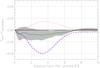 |
Fig. 1 Normalised intensity of 3C 454.3 subtracted from the normalised intensity of the object PSFs, as a function of distance from the PSF centroid. The reference profile is the PSF of quasar 3C 454.3 (black solid (0, 0) line). The calibrator star profile (blue dashed line) is the narrowest. The Vesta PSF (dashed magenta) is wider than the calibrator star, but still narrower than the reference PSF. The filled grey area represents the uncertainty of the nine Pluto observations. The mean median (MM) Pluto profile is shown as the green solid line. The most realistic dust ring model detected at 3σ significance level is plotted as the red dotted line. |
For each epoch a synthetic Pluto PSF was constructed using the combined quasar PSF as template. The synthetic Pluto PSF has two components, one corresponding to Pluto itself, the other describing the contribution of Charon (see Eq. (1)). The relative positions of these two bodies were taken from the Horizons database, as listed in Table A.1 and as presented in Fig. A.1. In the high spatial resolution model images, the two sources are placed in these relative positions. The relative contribution of Pluto and Charon to the total flux are characterised by the X ratio:  where Fq is the normalised synthetic quasar PSF, and x0 and y0 are the offsets of Charon’s position with respect to Pluto. The original, high-resolution image is convolved with the synthetic quasar PSF to obtain an “observable” model PSF. Because of the rotational variability of the surface of Pluto and Charon, the relative strength of the thermal fluxes cannot be determined very accurately, but their ratio is close to 2:1 or 3:1 depending on the model of their thermal properties (Lellouch et al. 2011). In our investigation we used both ratios, i.e. X = 0.67 and X = 0.75, respectively. The radial intensity profiles of the synthetic Pluto+Charon PSFs agree with each other very closely, indicating that the position and relative contribution of Charon to the total flux of the system has a minor effect on the intensity profile. This is mainly driven by the fact that Charon is very close to Pluto (06−08) compared to the size of the PSF in this band (57). In this respect, the difference observed between the radial intensity curves of the individual Pluto observations should mostly be attributed to measurement uncertainties. Therefore we constructed a mean measured (MM) radial intensity curve of the nine Pluto measurements, using equal weights in the case of all measurements. (The integration times and other conditions were the same for all measurements.)
The agreement of the model and observed curves are characterised by the reduced χ2-value: 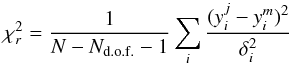 (1)where N is the number of data points, Nd.o.f. is the degrees of freedom,
  -s are the normalised intensity of the jth model at i distance, and
  are the median observed normalised intensities. The δi values are the standard deviations of the observed normalised intensities at a specific radial distance.
4. Intensity profile results
When the MM curve of Pluto is compared with the mean synthetic (MS) curve of the nine epochs, we obtain a difference with a low level of significance (0.8σ) between radial distances 0′′−22′′. This shows that the observed Pluto PSFs are very similar to the synthetic ones and that we are not able to detect any extended emission feature around Pluto, i.e. there is no obvious evidence of a notable dust ring in the Pluto–Charon system.
It is, however, an important question about what the total brightness of such a hypothetical disk/ring could be that would still be detectable with our method. To test this, we constructed a set of model images, in each case placing a ring in addition to the contributions of Pluto and Charon, as described above. The moons of the Pluto system seem to revolve in a well-defined plane, so that any stable ring/disk is expected in this plane with the highest probability (Nagy et al. 2006). We model the ring as a surface brightness enhancement around a specific distance (r0) from the barycentre of the Pluto-Charon system in the midplane of the moon system (tilted w.r.t. the line of sight by an orientation angle of 61°), assuming a Gaussian intensity profile in the surface brightness distribution. The parameters characterising the surface brightness of the ring are (i) r0, the distance of the ring from the barycentre; (ii) the width of the Gaussian Δr and (iii) Fr, the total flux density of the ring. We constructed model images using these parameters in the range Fr = 0−60 mJy, r0 = 2.55 × 10⁴ − 1.53× 10⁵ km (11−66), and Δr = 1.16 × 10⁴, 1.74 × 10⁴, and 2.32 × 10⁴ km (05, 075 and 10). For each model we calculated the  of the difference. The F0 (ring excess) dependence of the values corresponding to the 1σ and 3σ significance levels are presented in Fig. 2, where σ is the standard deviation of the χ2 distribution.
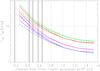 |
Fig. 2 F0 (ring excess) values as a function of distance from the Pluto–Charon barycentre. Red and green colours correspond to FPluto and FCharon ratio of 2:1 and 3:1, for 3σ significance. Blue and magenta colours refer to the same ratios, but for 1σ. Solid, dashed, and dashed-dotted lines represent the width of the modelled ring Δr = 0 |
Figure 2 shows that our method is the most sensitive at higher radial distances, and the detection probability also depends on the X flux ratio. In the case of rings close to Pluto, the detection limit is significantly higher; for example, at the distance of Charon, we would only be able to detect a ring with ~100 mJy excess, therefore we are not able to constrain the presence or lack of a ring within or close to the orbit of Charon. The lowest detection limit belongs to X = 0.67 with ring distance of 66, in this case F(1σ) = 1.8 mJy and F(3σ) = 3.3 mJy.
A possible dust ring around the Pluto–Charon system is expected to be in the region where the satellites exist. We assume that the most realistic model is where X = 0.67, r0 = 22 (5.1 × 10⁴ km), and Δr = 10 (2.32 × 10⁴ km). In this case the ring is centred on a distance between Kerberos and Nix, and the ring Δr also models an extended feature where 58% exists inside the orbit of the Pluto satellites. The results show that for this ring configuration, we obtain F0 = 6.0 and 10.8 mJy for the 1σ and 3σ significance levels, respectively. This implies that the detection probability for this geometry is ~68% for a ring with 6.0 mJy total flux density and 99.7% with 10.8 mJy.
5. Discussion
Our method is able to detect infrared excess from a ring according to Fig. 2. Any calculation that wants to derive dust surface density or impactor mass based on this excess has to rely on assumptions about the type and the spatial and grain size distribution of the dust.
Assuming that the material of our hypothetical ring is dominated by grains that are in thermal equilibrium with the solar radiation, we can give a rough estimate of the mass of this ring. Considering a black body temperature of Td = 278.3× (r/ 1 [ au ] )− 1 / 2 = 48.9 K (Kennedy & Wyatt 2011) and an absorption coefficient of κabs = 5.96 m2 kg-1 at 70 μm (Li & Draine 2001), we can estimate the dust mass according to Eq. (2) below: ![Mathematical equation: \begin{equation} M_{\rm dust}=\frac{\Delta^2 F_{\nu}(\lambda)}{\kappa_{\rm abs} B_{\nu}(\lambda,T)} = 2.28\times10^{9}\times\frac{F_{70}(\lambda)}{\rm mJy}~[{\rm kg}], \label{eq3} \end{equation}](/articles/aa/full_html/2015/07/aa25668-15/aa25668-15-eq59.png) (2)where Δ is the distance to the observer, and Bν(Td) the Planck function. Applying Eq. (2) to the most realistic case put forward in Sect. 4, the 3σ flux limit is 10.8 mJy, and we obtain a total disk mass of 2.5 × 10¹⁰ kg, which is equivalent to the mass of a ~340 m-sized small body when assuming an average density of ρ = 1.2 g cm-3.
(2)where Δ is the distance to the observer, and Bν(Td) the Planck function. Applying Eq. (2) to the most realistic case put forward in Sect. 4, the 3σ flux limit is 10.8 mJy, and we obtain a total disk mass of 2.5 × 10¹⁰ kg, which is equivalent to the mass of a ~340 m-sized small body when assuming an average density of ρ = 1.2 g cm-3.
The fly-by of New Horizons is planned to take place inside the Charon orbit. Taking the maximum separation of 085 between Pluto and Charon, we calculated the amount of mass and the corresponding surface density for the area between the two objects. The fraction of the total ring dust mass located within 085 is 4.3 × 10⁻⁴ (1.1 × 10⁷ kg). This corresponds to a surface density of 8.7 × 10⁻¹⁰ g cm-2 and an impactor mass of ~8.7 × 10⁻⁵ g. This is very similar, only ~10% lower, to the impactor mass of 10-4 g obtained by Steffl & Stern (2007) based on Hubble Space Telescope observations. We note that a thinner ring with the same brightness would result in a significantly lower impactor mass.
6. Summary
In this paper we searched for far-infrared signatures of a possible dust ring around the Pluto–Charon system.
We found no clear observational evidence of a dust ring, but we were able to put model-dependent upper limits on the
possible amount of dust emission that could remain undetectable by our method. For a realistic ring configuration, we put a 3σ upper flux density limit of 10.8 mJy at 70 μm. This corresponds to a surface density of 8.7 × 10⁻¹⁰ g cm-2 in the region between Pluto and Charon. Our estimated impactor mass for the New Horizons fly-by is very similar (~ 10% lower) to the previous results of Steffl & Stern (2007), and it suggests that the satellite will not be endangered by particle collisions.
Online material
Appendix A: Basic properties of the Pluto–Charon Herschel observations
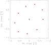 |
Fig. A.1 Position of Charon (red rhombs) at the time of the observations relative to Pluto (black plus sign). |
Basic properties of the Pluto–Charon Herschel observations.
Appendix B: Modelled total ring flux values
Total flux values of model rings of different configurations.
Appendix C: PSF profiles
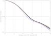 |
Fig. C.1 Normalised intensity profiles as a function of distance from the PSF centroid. The quasar 3C 454.3 is shown with a black solid line. The calibrator star profile is presented with a blue dashed line. The dashed-dotted magenta line indicates the Vesta PSF. The solid green line shows the mean of the nine Pluto observations (MM), while the filled grey area represents the measurement uncertainty. The faintest dust ring model detected at 3σ significance level is plotted with a dotted red line. |
http://herschel.esac.esa.int/hpt/publicationdetailsview.do? bibcode=2012ApJ...758...72W.
Acknowledgments
We thank our anonymous referee for the useful comments that helped to improve the content of the paper. This work has been supported by the PECS contract # 4000109997/13/NL/KML of the Hungarian Space Office and the European Space Agency by and the Hungarian Research Fund (OTKA) grants Nos. 101939 and 104607.
References
- Balog, Z., Müller, T. G., Nielbock, M., et al. 2014, Exp. Astron., 37, 129 [NASA ADS] [CrossRef] [EDP Sciences] [Google Scholar]
- Boissel, Y., Sicardy, B., Roques, F., et al. 2014, A&A, 561, A144 [NASA ADS] [CrossRef] [EDP Sciences] [Google Scholar]
- Braga-Ribas, F., Sicardy, B., Ortiz, J. L., et al. 2014, Nature, 508, 72 [NASA ADS] [CrossRef] [Google Scholar]
- Buie, M. W., Grundy, W. M., Young, E. F., et al. 2006, AJ, 132, 290 [NASA ADS] [CrossRef] [Google Scholar]
- Durda, D. D., & Stern, S. A. 2000, Icarus, 145, 220 [Google Scholar]
- Giuliatti Winter, S. M., Winter, O. C., Guimares, A. H., & Silva, M. R. 2010, MNRAS, 404, 442 [NASA ADS] [Google Scholar]
- Giuliatti Winter, S. M., Winter, O. C., Vieira Neto, E., & Sfair, R. 2013, MNRAS, 430, 1892 [NASA ADS] [CrossRef] [Google Scholar]
- Kennedy, G. M., & Wyatt, M. C. 2011, MNRAS, 412, 2137 [NASA ADS] [CrossRef] [Google Scholar]
- Karkoschka, E. 2001, Icarus, 151, 51 [NASA ADS] [CrossRef] [Google Scholar]
- Li, A., & Draine, B. T. 2001, ApJ, 554, 778 [Google Scholar]
- Lellouch, E., Stansberry, J., & Emery, J. 2011, Icarus, 214, 701 [NASA ADS] [CrossRef] [Google Scholar]
- Lellouch, E., Santos-Sanz, P., Fornasier, S., et al. 2013, EPSC2013-91, London, 9–13 Sept. [Google Scholar]
- Lutz, D. 2012, PICC-ME-TN-033 [Google Scholar]
- Moór, A., Müller, T. G., Kiss, C., et al. 2014, Exp. Astron., 37, 225 [NASA ADS] [CrossRef] [Google Scholar]
- Moór, A., Kóspál, Á., Ábrahám, P., et al. 2015, MNRAS, 447, 577 [NASA ADS] [CrossRef] [Google Scholar]
- Nagy, I., Süli, Á., & Érdi, B. 2006, MNRAS, 370, 19 [NASA ADS] [CrossRef] [Google Scholar]
- Ortiz, J. L., Duffard, R., Pinilla-Alonso, N., et al. 2015, A&A, 576, A18 [NASA ADS] [CrossRef] [EDP Sciences] [Google Scholar]
- Ott, S. 2010, ASP Conf. Ser., 434, 139 [Google Scholar]
- Paladini, R., Ali, B., Altieri, B., et al. 2013, PACS mapmaking report [Google Scholar]
- Pilbratt, G. L., Riedinger, J. R., Passvogel, T., et al. 2010, A&A, 518, A1 [NASA ADS] [CrossRef] [EDP Sciences] [Google Scholar]
- Pires Dos Santos, P. M., Giuliatti Winter, S. M., & Sfair, R. 2011, MNRAS, 410, 273 [NASA ADS] [CrossRef] [Google Scholar]
- Poglitsch, A., Waelkens, C., Geis, N., et al. 2010, A&A, 518, A2 [Google Scholar]
- Popesso, P., Magnelli, B., Buttiglione, S., et al. 2011, A&A, submitted [arXiv:1211.4257] [Google Scholar]
- Showalter, M. R., Hamilton, D. P., Stern, S. A., et al. 2011, CBET, 2769, 1 [NASA ADS] [Google Scholar]
- Showalter, M. R., Weaver, H. A., Stern, S. A., et al. 2012, CBET, 9253, 1 [Google Scholar]
- Steffl, A. J., & Stern, S. A. 2007, AJ, 133, 1485 [NASA ADS] [CrossRef] [Google Scholar]
- Steffl, A. J., Mutchler, M. J., Weaver, H. A., et al. 2006, AJ, 132, 614 [NASA ADS] [CrossRef] [Google Scholar]
- Stern, S. A. 2008, Space Sci. Rev., 140, 3 [NASA ADS] [CrossRef] [Google Scholar]
- Süli, Á., & Zsigmond, Zs. 2009, MNRAS, 398, 2199 [NASA ADS] [CrossRef] [Google Scholar]
- Weaver, H. A., Stern, S. A., Mutchler, M. J., et al. 2006, Nature, 439, 943 [NASA ADS] [CrossRef] [Google Scholar]
- Wehrle, A. E., Marscher, A. P., Jorstad, S. G., et al. 2012, ApJ, 758, 72 [NASA ADS] [CrossRef] [Google Scholar]
- Zsigmond, Zs., & Süli, Á. 2010, J. Phys. Conf. Ser., 218, 2020 [NASA ADS] [CrossRef] [Google Scholar]
All Tables
All Figures
|
Fig. 1 Normalised intensity of 3C 454.3 subtracted from the normalised intensity of the object PSFs, as a function of distance from the PSF centroid. The reference profile is the PSF of quasar 3C 454.3 (black solid (0, 0) line). The calibrator star profile (blue dashed line) is the narrowest. The Vesta PSF (dashed magenta) is wider than the calibrator star, but still narrower than the reference PSF. The filled grey area represents the uncertainty of the nine Pluto observations. The mean median (MM) Pluto profile is shown as the green solid line. The most realistic dust ring model detected at 3σ significance level is plotted as the red dotted line. |
| In the text | |
|
Fig. 2 F0 (ring excess) values as a function of distance from the Pluto–Charon barycentre. Red and green colours correspond to FPluto and FCharon ratio of 2:1 and 3:1, for 3σ significance. Blue and magenta colours refer to the same ratios, but for 1σ. Solid, dashed, and dashed-dotted lines represent the width of the modelled ring Δr = 0 |
| In the text | |
|
Fig. A.1 Position of Charon (red rhombs) at the time of the observations relative to Pluto (black plus sign). |
| In the text | |
|
Fig. C.1 Normalised intensity profiles as a function of distance from the PSF centroid. The quasar 3C 454.3 is shown with a black solid line. The calibrator star profile is presented with a blue dashed line. The dashed-dotted magenta line indicates the Vesta PSF. The solid green line shows the mean of the nine Pluto observations (MM), while the filled grey area represents the measurement uncertainty. The faintest dust ring model detected at 3σ significance level is plotted with a dotted red line. |
| In the text | |
Current usage metrics show cumulative count of Article Views (full-text article views including HTML views, PDF and ePub downloads, according to the available data) and Abstracts Views on Vision4Press platform.
Data correspond to usage on the plateform after 2015. The current usage metrics is available 48-96 hours after online publication and is updated daily on week days.
Initial download of the metrics may take a while.