© ESO, 2015

1. Introduction

Most astrophysical shocks, whether in the solar system, in the interstellar medium, or very large scale shocks in clusters of galaxies, are so-called collisionless shocks. The change in flow and plasma parameters across these shocks are not established through particle-particle collisions (Coulomb interactions), but through collective effects (electric and magnetic field fluctuations, see the textbooks devoted to collisionless shocks by Tidman & Krall 1971; Balogh & Treumann 2013). One of the questions about collisionless shocks is whether or not different types of particles will be shock-heated to the same temperature or not. For a high Mach number shock in a single fluid approximation characterised by an adiabatic index of γ = 5/3 the post-shock temperature should, according to the Rankine-Hugoniot jump conditions, be 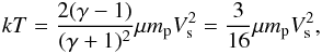$\begin{array}{ccc}\mathit{kT}\mathrm{=}\frac{\mathrm{2}\mathrm{(}\mathit{\gamma }\mathrm{-}\mathrm{1}\mathrm{)}}{\mathrm{(}\mathit{\gamma }\mathrm{+}\mathrm{1}{\mathrm{)}}^{\mathrm{2}}}\mathit{\mu }{\mathit{m}}_{\mathrm{p}}{\mathit{V}}_{\mathrm{s}}^{\mathrm{2}}\mathrm{=}\frac{\mathrm{3}}{\mathrm{16}}\mathit{\mu }{\mathit{m}}_{\mathrm{p}}{\mathit{V}}_{\mathrm{s}}^{\mathrm{2}}\mathit{,}& & \end{array}$(1)with μ the average mass of the particles in units of the proton mass m_p, and V_s the shock velocity. For plasmas with solar abundances μ ≈ 0.6¹. For collisionless shock heating, i.e. in absence of Coulomb equilibration, it is not clear whether a single temperature kT characterises the temperature of each particle species, since this requires equilibration of energies between the ions and the electrons. It is not a priori known how this equilibration should be established, since electron-ion collisions are by definition negligible in collisionless shocks. Instead it is often assumed that downstream of high Mach number, collisionless shocks the expected temperature for each species i is given by 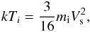$\begin{array}{ccc}\mathit{k}{\mathit{T}}_{\mathit{i}}\mathrm{=}\frac{\mathrm{3}}{\mathrm{16}}{\mathit{m}}_{\mathrm{i}}{\mathit{V}}_{\mathrm{s}}^{\mathrm{2}}\mathit{,}& & \end{array}$(2)which implies that electrons have a temperature a factor 1/1836 lower than the protons (e.g. Ghavamian et al. 2013, for review). Note that further downstream of the shock Coulomb collisions will tend to slowly equilibrate the ion and electron temperatures. But plasmas in objects like young supernova remnants (SNRs) are likely not to have reached full temperature equilibrium throughout the entire shell (Itoh 1978; Vink 2012; Ghavamian et al. 2013). The non-equilibration of ion and electron temperatures is not only important for SNRs, but appears also to affect low Mach number shocks in the solar system (e.g. Schwartz et al. 1988), clusters of galaxies (Russell et al. 2012), and may affect the observability of the yet to be detected warm hot intergalactic medium (WHIM, Bykov et al. 2008), in which a fraction of 40–50% of the baryons in the Universe reside.

Clear observational evidence for non-equilibration of electron and ion temperatures comes from SNRs. Early evidence for non-equilibration was provided by the fact that young SNRs seem to have lower electron temperatures (kT_e ≲ 4 keV) than they should have given that they have shock speeds up to ~5000 km s^-1 (kT ~ 30 keV). More direct proof that SNR shocks heat the electrons to lower temperatures than the ions comes from measurements of the ion temperatures, obtained from thermal Doppler broadening of line emission in the optical (Rakowski et al. 2003; Ghavamian et al. 2007), UV (Raymond et al. 1995), and X-rays (Vink et al. 2003; Furuzawa et al. 2009; Broersen et al. 2013). The most extensive results come from optical spectroscopy, using the broad-line component of Hα emission, which arises from charge exchange between neutral hydrogen penetrating the shock and already shock-heated protons downstream of the shock. The ratio between the narrow-line Hα component, caused by direct excitation, and the broad-line component is sensitive to the ratio of the electron to ion temperature (Ghavamian et al. 2007; van Adelsberg et al. 2008). In some cases broad-line Hα measurements can be supplemented by X-ray measurements of the electron temperature (Rakowski et al. 2003; Helder et al. 2011). These measurements suggest that for shock velocities ≲400 km s^-1 the electron and proton temperatures are more or less equal, whereas for higher velocities the degree of equilibration appears to decrease roughly as T_e/T_p ∝ V^-2 (Ghavamian et al. 2007).

Observations of electron heating at the Earth bowshock shows that electrons are in most cases heated to lower temperatures than the ions (Schwartz et al. 1988), with a Mach number dependence that suggests that there is an inverse correlation between Mach number and electron-ion temperature ratio (Ghavamian et al. 2013). Finally, measurements of post-shock temperature profiles in clusters of galaxies indicate that the electrons are heated at the shock to similar temperatures as the ions (Markevitch 2006), or they obtain slightly lower temperatures than the ions (Russell et al. 2012).

In this paper we provide an alternative, simple explanation for the behaviour of the electron-ion equilibration as a function of Mach number. The approach does not rely on details of the shock heating mechanism itself, but only on the thermodynamics of the shocks. The only assumption that is made is that the density jump across the shock is the same for all species, in order to maintain charge neutrality. We show that this assumption does not support the sometimes expressed idea that non-equilibration implies that T_e/T_i ≈ m_e/m_i. Instead we show that for low Mach numbers T_e/T_i ≈ 1, and that only for high Mach numbers T_e/T_i = m_e/m_i. In between these extremes we obtain a relation T_e/T_p ∝ M^-2, similar to the relation suggested by Ghavamian et al. (2007). A further modification to the model is made by parameterising ion-electron heat exchange, heuristically allowing for additional heat flow from the ions to the electrons.

2. Derivation of a relation between electron and ion temperatures

The shock jump conditions for a plane parallel unmagnetised shock are given by the well known Rankine-Hugoniot relations 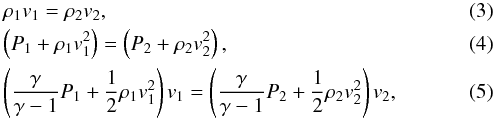$\begin{array}{ccc}& & \\ & & \\ & & \end{array}$with the subscripts 1 and 2 indicating the quantities upstream and downstream of the shock respectively, v the plasma velocity in the frame comoving with the shock, ρ = nμm_p the density (and with n the particle density), and P = nkT the gas pressure. The solution to this equation is that the density ratio between pre-shock and post-shock plasma is $\begin{array}{ccc}\mathit{\chi }\mathrm{\equiv }\frac{{\mathit{\rho }}_{\mathrm{2}}}{{\mathit{\rho }}_{\mathrm{1}}}\mathrm{=}\frac{{\mathit{v}}_{\mathrm{1}}}{{\mathit{v}}_{\mathrm{2}}}\mathrm{=}\frac{\mathrm{(}\mathit{\gamma }\mathrm{+}\mathrm{1}\mathrm{)}{\mathit{M}}_{\mathrm{s}}^{\mathrm{2}}}{\mathrm{(}\mathit{\gamma }\mathrm{-}\mathrm{1}\mathrm{)}{\mathit{M}}_{\mathrm{s}}^{\mathrm{2}}\mathrm{+}\mathrm{2}}\mathit{,}& & \end{array}$(6)and that the downstream temperature is $\begin{array}{ccc}\mathit{k}{\mathit{T}}_{\mathrm{2}}\mathrm{=}\frac{\mathrm{1}}{\mathit{\chi }}\left[\frac{\mathrm{1}}{\mathit{\gamma }{\mathit{M}}_{\mathrm{s}}^{\mathrm{2}}}\mathrm{+}\left(\mathrm{1}\mathrm{-}\frac{\mathrm{1}}{\mathit{\chi }}\right)\right]\mathit{\mu }{\mathit{m}}_{\mathrm{p}}{\mathit{v}}_{\mathrm{1}}^{\mathrm{2}}\mathit{,}& & \end{array}$(7)with γ = 5/3 the adiabatic index, and ${\mathit{M}}_{\mathrm{s}}\mathrm{\equiv }{\mathit{v}}_{\mathrm{1}}\mathit{/}{\mathit{c}}_{\mathrm{s}}\mathrm{=}\sqrt{\mathit{\rho }{\mathit{v}}_{\mathrm{1}}^{\mathrm{2}}\mathit{/}\mathrm{\left(}\mathit{\gamma }{\mathit{P}}_{\mathrm{1}}\mathrm{\right)}}$ the sonic shock Mach number. For M_s → ∞ this becomes Eq. (1). In Sect. 2.3 we also discuss the effects of magnetic fields, in which case the Alfvén Mach number should also be taken into account.

Note that these solutions do not take into account the effects of cosmic-ray acceleration. Cosmic-ray acceleration can be taken into account in the framework of the Rankine-Hugoniot relations (e.g. Vink et al. 2010), by allowing for compression of the inflowing plasma caused by interactions with cosmic rays in a so-called cosmic-ray precursor. In that case the actual gas shock, called sub-shock, will have a lower Mach number than the overal Mach number, as the inflowing plasma has already been heated by adiabatic compression or even non-adiabatic heating processes, operating in the shock precursor. Equations (3)–(5) should then be applied to the sub-shock alone, and also the relations we derive below should be strictly applied to the sub-shock, and not to the overall shock structure (sub-shock plus cosmic-ray precursor region).

Applying the full shock jump relations to each particle species separately would lead to both separate temperatures and to separate shock compression ratios χ. Although separate temperatures are to be expected for collisionless shocks, separate compression ratios are very unlikely, as it would lead to charge separation, and hence large scale electric fields. The length scale over which charge separation is dissolved is typically of the order of the Debye length ${\mathit{l}}_{\mathrm{D}}\mathrm{\approx }\sqrt{\mathit{kT}\mathit{/}\mathrm{\left(}\mathrm{4}\mathit{\pi }{\mathit{n}}_{\mathrm{e}}{\mathit{e}}^{\mathrm{2}}\mathrm{\right)}}\mathrm{\approx }\mathrm{0.22}{\mathit{n}}_{\mathrm{e}}^{\mathrm{-}\mathrm{1}\mathit{/}\mathrm{2}}\mathrm{(}\mathit{T}\mathit{/}{\mathrm{10}}^{\mathrm{7}}\hspace{0.17em}\mathrm{K}{\mathrm{)}}^{\mathrm{1}\mathit{/}\mathrm{2}}$ km, which indicates the distance over which the electric potential energy equals the kinetic energy of the charge particles (e.g. Zel’dovich & Raizer 1966; Spitzer 1965). The Debye length is much smaller than the typical length scale over which the shock is established, ${\mathit{l}}_{\mathrm{sh}}\mathrm{\approx }\mathit{c}\mathit{/}{\mathit{\omega }}_{\mathrm{pi}}\mathrm{=}\sqrt{{\mathit{c}}^{\mathrm{2}}{\mathit{m}}_{\mathrm{p}}\mathit{/}\mathrm{\left(}\mathrm{4}\mathit{\pi }{\mathit{n}}_{\mathrm{i}}{\mathit{e}}^{\mathrm{2}}\mathrm{\right)}}\mathrm{\approx }\mathrm{228}{\mathit{n}}_{\mathrm{i}}^{\mathrm{-}\mathrm{1}\mathit{/}\mathrm{2}}$ km (e.g. Bale et al. 2003). The ratio of these two length scales is ${\mathit{l}}_{\mathrm{D}}\mathit{/}{\mathit{l}}_{\mathrm{sh}}\mathrm{=}\sqrt{\mathit{kT}\mathit{/}\mathrm{\left(}{\mathit{m}}_{\mathrm{p}}{\mathit{c}}^{\mathrm{2}}\mathrm{\right)}}$, which for non-relativistic shocks is much lower than one.

The most natural outcome of a collisionless shock seems, therefore, that the overall shock jump conditions should be applied to the plasma as a whole, leading to only one value for the compression ratio, χ = ρ₂/ρ₁ = ρ_e,2/ρ_e,1 = ρ_i,2/ρ_i,1, with the indices e and i indicating respectively the electron and ion contributions. This implies that we apply only Eqs. (4) and (5) to the particle species separately, as Eq. (3) is already determined by the full set of jump conditions applied to the plasma as a whole. Of the two remaining equations, it seems more natural to concentrate on the enthalpy-flux conservation (Eq. (5)) for each separate species, because electrons and ions can easily change directions, influencing the individual momenta of the particles (momentum being a vector) whereas the energy exchange between species is absent or very slow in collisionless plasmas. In other words, we do expect some exchange of momentum between electrons and ions (mediated by the electromagnetic field at the shock), whereas energy exchange between electrons and ions is more difficult. This implies that the enthalpy flux of each particle species is conserved separately, but that not necessarily the momentum flux of each species is conserved separately. An analogy that comes to mind is a ball bouncing elastically off a wall. The lightest of the objects in that case, the ball, preserves its kinetic energy, but the momentum has clearly changed (the ball reversed its direction). Considering only Eq. (5) for each separate species implies that the heating of electrons is simply caused by redistribution and thermalisation of the energy of the electrons, perhaps through elastic scatterings in the shock regions, followed by electron-electron equilibration.

To calculate what the effects are of this ansatz, it is useful to introduce the following relations between temperature and sonic Mach numbers: $\begin{array}{ccc}\frac{\mathit{k}{\mathit{T}}_{\mathrm{1}}}{\mathit{\mu }{\mathit{m}}_{\mathrm{p}}{\mathit{v}}_{\mathrm{1}}^{\mathrm{2}}}\mathrm{=}\frac{{\mathit{P}}_{\mathrm{1}}}{{\mathit{\rho }}_{\mathrm{1}}{\mathit{v}}_{\mathrm{1}}^{\mathrm{2}}}\mathrm{=}\frac{\mathrm{1}}{\mathit{\gamma }{\mathit{M}}_{\mathrm{s}}^{\mathrm{2}}}\mathit{,}\frac{\mathit{k}{\mathit{T}}_{\mathrm{1}}}{{\mathit{\mu }}_{\mathrm{e}}{\mathit{m}}_{\mathrm{p}}{\mathit{v}}_{\mathrm{1}}^{\mathrm{2}}}\mathrm{=}\left(\frac{\mathit{\mu }}{{\mathit{\mu }}_{\mathrm{e}}}\right)\frac{\mathrm{1}}{\mathit{\gamma }{\mathit{M}}_{\mathrm{s}}^{\mathrm{2}}}\mathit{,}\frac{\mathit{k}{\mathit{T}}_{\mathrm{1}}}{{\mathit{\mu }}_{\mathrm{i}}{\mathit{m}}_{\mathrm{p}}{\mathit{v}}_{\mathrm{1}}^{\mathrm{2}}}\mathrm{=}\left(\frac{\mathit{\mu }}{{\mathit{\mu }}_{\mathrm{i}}}\right)\frac{\mathrm{1}}{\mathit{\gamma }{\mathit{M}}_{\mathrm{s}}^{\mathrm{2}}}\mathit{,}& & \end{array}$(8)where we have used the notation that μ is the average mass of all species in units of the proton mass, whereas μ_e (=m_e/m_p ≈ 1/1836) is the electron mass and μ_i the average ion mass (protons and other ions) in units of the proton mass. For solar abundance plasmas μ_i ≈ 1.27.

2.1. The most extreme case of non-equilibration of electron and ion temperatures

We now proceed by considering the electron-enthalpy flux separately: $\begin{array}{ccc}\left(\frac{\mathit{\gamma }}{\mathit{\gamma }\mathrm{-}\mathrm{1}}{\mathit{P}}_{\mathrm{e}\mathit{,}\mathrm{2}}\mathrm{+}\frac{\mathrm{1}}{\mathrm{2}}{\mathit{\rho }}_{\mathrm{e}\mathit{,}\mathrm{2}}{\mathit{v}}_{\mathrm{2}}^{\mathrm{2}}\right){\mathit{v}}_{\mathrm{2}}\mathrm{=}\left(\frac{\mathit{\gamma }}{\mathit{\gamma }\mathrm{-}\mathrm{1}}{\mathit{P}}_{\mathrm{e}\mathit{,}\mathrm{1}}\mathrm{+}\frac{\mathrm{1}}{\mathrm{2}}{\mathit{\rho }}_{\mathrm{e}\mathit{,}\mathrm{1}}{\mathit{v}}_{\mathrm{1}}^{\mathrm{2}}\right){\mathit{v}}_{\mathrm{1}}\mathit{.}& & \end{array}$(9)Note that we assume that the electrons and ions have equal bulk velocities. The downstream electron temperature kT_e,2 is contained in the pressure term, P_e,2 = n_e,2kT_e,2. With the help of Eq. (8), and assuming that the electrons and ions are equilibrated upstream of the shock (i.e. kT_e,1 = kT_i,1 = kT₁), we obtain $\begin{array}{ccc}\frac{\mathit{k}{\mathit{T}}_{\mathrm{e}\mathit{,}\mathrm{2}}}{{\mathit{\mu }}_{\mathrm{e}}{\mathit{m}}_{\mathrm{p}}{\mathit{v}}_{\mathrm{1}}^{\mathrm{2}}}\mathrm{=}\frac{\mathit{k}{\mathit{T}}_{\mathrm{e}\mathit{,}\mathrm{1}}}{{\mathit{\mu }}_{\mathrm{e}}{\mathit{m}}_{\mathrm{p}}{\mathit{v}}_{\mathrm{1}}^{\mathrm{2}}}\mathrm{+}\frac{\mathrm{1}}{\mathrm{2}}\left(\frac{\mathit{\gamma }\mathrm{-}\mathrm{1}}{\mathit{\gamma }}\right)\left(\mathrm{1}\mathrm{-}\frac{\mathrm{1}}{{\mathit{\chi }}^{\mathrm{2}}}\right)\mathrm{=}\frac{\mathrm{1}}{\mathit{\gamma }{\mathit{M}}_{\mathrm{s}}^{\mathrm{2}}}\left(\frac{\mathit{\mu }}{{\mathit{\mu }}_{\mathrm{e}}}\right)\mathrm{+}\frac{\mathrm{1}}{\mathrm{2}}\left(\frac{\mathit{\gamma }\mathrm{-}\mathrm{1}}{\mathit{\gamma }}\right)\left(\mathrm{1}\mathrm{-}\frac{\mathrm{1}}{{\mathit{\chi }}^{\mathrm{2}}}\right)\mathit{,}& & \end{array}$(10)which for γ = 5/3,M_s → ∞ (implying χ = 4) gives $\begin{array}{ccc}\mathit{k}{\mathit{T}}_{\mathrm{e}\mathit{,}\mathrm{2}}\mathrm{=}\frac{\mathrm{1}}{\mathrm{2}}\left(\frac{\mathit{\gamma }\mathrm{-}\mathrm{1}}{\mathit{\gamma }}\right)\left(\mathrm{1}\mathrm{-}\frac{\mathrm{1}}{{\mathit{\chi }}^{\mathrm{2}}}\right){\mathit{\mu }}_{\mathrm{e}}{\mathit{m}}_{\mathrm{p}}{\mathit{v}}_{\mathrm{1}}^{\mathrm{2}}\mathrm{=}\frac{\mathrm{3}}{\mathrm{16}}{\mathit{\mu }}_{\mathrm{e}}{\mathit{m}}_{\mathrm{p}}{\mathit{v}}_{\mathrm{1}}^{\mathrm{2}}\mathit{,}& & \end{array}$(11)which is the expected temperature if there is no electron-ion equilibration established by the shock.

In a similar way we can calculate the downstream ion temperature by assuming ion-enthalpy flux conservation: $\begin{array}{ccc}\frac{\mathit{k}{\mathit{T}}_{\mathrm{i}\mathit{,}\mathrm{2}}}{{\mathit{\mu }}_{\mathrm{i}}{\mathit{m}}_{\mathrm{p}}{\mathit{v}}_{\mathrm{1}}^{\mathrm{2}}}\mathrm{=}\frac{\mathit{k}{\mathit{T}}_{\mathrm{i}\mathit{,}\mathrm{1}}}{{\mathit{\mu }}_{\mathrm{i}}{\mathit{m}}_{\mathrm{p}}{\mathit{v}}_{\mathrm{1}}^{\mathrm{2}}}\mathrm{+}\frac{\mathrm{1}}{\mathrm{2}}\left(\frac{\mathit{\gamma }\mathrm{-}\mathrm{1}}{\mathit{\gamma }}\right)\left(\mathrm{1}\mathrm{-}\frac{\mathrm{1}}{{\mathit{\chi }}^{\mathrm{2}}}\right)\mathrm{=}\frac{\mathrm{1}}{\mathit{\gamma }{\mathit{M}}_{\mathrm{s}}^{\mathrm{2}}}\left(\frac{\mathit{\mu }}{{\mathit{\mu }}_{\mathrm{i}}}\right)\mathrm{+}\frac{\mathrm{1}}{\mathrm{2}}\left(\frac{\mathit{\gamma }\mathrm{-}\mathrm{1}}{\mathit{\gamma }}\right)\left(\mathrm{1}\mathrm{-}\frac{\mathrm{1}}{{\mathit{\chi }}^{\mathrm{2}}}\right)\mathrm{·}& & \end{array}$(12)Combining Eq. (10) with Eq. (12) we see that the ratio of the electron temperature over ion temperature is $\begin{array}{ccc}\frac{{\mathit{T}}_{\mathrm{e}\mathit{,}\mathrm{2}}}{{\mathit{T}}_{\mathrm{i}\mathit{,}\mathrm{2}}}\mathrm{=}\left(\frac{{\mathit{\mu }}_{\mathrm{e}}}{{\mathit{\mu }}_{\mathrm{i}}}\right)\frac{\mathrm{2}\left(\frac{\mathit{\mu }}{{\mathit{\mu }}_{\mathrm{e}}}\right){\mathit{\chi }}^{\mathrm{2}}\mathrm{+}{\mathit{M}}_{\mathrm{s}}^{\mathrm{2}}\mathrm{(}\mathit{\gamma }\mathrm{-}\mathrm{1}\mathrm{)}\mathrm{(}{\mathit{\chi }}^{\mathrm{2}}\mathrm{-}\mathrm{1}\mathrm{)}}{\mathrm{2}\left(\frac{\mathit{\mu }}{{\mathit{\mu }}_{\mathrm{i}}}\right){\mathit{\chi }}^{\mathrm{2}}\mathrm{+}{\mathit{M}}_{\mathrm{s}}^{\mathrm{2}}\mathrm{(}\mathit{\gamma }\mathrm{-}\mathrm{1}\mathrm{)}\mathrm{(}{\mathit{\chi }}^{\mathrm{2}}\mathrm{-}\mathrm{1}\mathrm{)}}\mathrm{·}& & \end{array}$(13)This relation is shown as a solid line in Fig. 1.

For M_s → ∞ we find that kT_e/kT_i = μ_e/μ_i, as usually proposed for extreme non-equilibration, whereas for M_s → 1,χ → 1, we obtain kT_e,2/kT_i,2 → 1. We see also that for $\begin{array}{ccc}\sqrt{\frac{\mathrm{2}}{\mathrm{(}\mathit{\gamma }\mathrm{-}\mathrm{1}\mathrm{)}}\frac{\mathit{\mu }}{{\mathit{\mu }}_{\mathrm{i}}}\left(\frac{{\mathit{\chi }}^{\mathrm{2}}}{{\mathit{\chi }}^{\mathrm{2}}\mathrm{-}\mathrm{1}}\right)}\mathit{<}{\mathit{M}}_{\mathrm{s}}\mathit{<}\sqrt{\frac{\mathrm{2}}{\mathrm{(}\mathit{\gamma }\mathrm{-}\mathrm{1}\mathrm{)}}\frac{\mathit{\mu }}{{\mathit{\mu }}_{\mathrm{e}}}\left(\frac{{\mathit{\chi }}^{\mathrm{2}}}{{\mathit{\chi }}^{\mathrm{2}}\mathrm{-}\mathrm{1}}\right)}& & \end{array}$(14)(approximately 2 <M_s< 60) the term with M_s in the denominator of Eq. (13) is dominant, whereas M_s is not yet important for the nominator. As a result the electron-ion temperature ratio in this range of M_s scales as $\mathit{k}{\mathit{T}}_{\mathrm{e}\mathit{,}\mathrm{2}}\mathit{/}\mathit{k}{\mathit{T}}_{\mathrm{i}\mathit{,}\mathrm{2}}\mathrm{\propto }\mathrm{1}\mathit{/}{\mathit{M}}_{\mathrm{s}}^{\mathrm{2}}$.

The result that the electron-electron-ion temperature ratios are close to one for low Mach numbers (M_s ≈ 1) and that the ratio decreases for higher Mach numbers, can be made intuitively clear by realising that at relatively low Mach numbers the enthalpy-flux is dominated by the pre-shock thermal energy, which is similar for the electrons and the ions (i.e. on average each particle has an energy of kT₁ irrespective of its mass). For high Mach numbers the enthalpy flux is dominated by the bulk motion of the particles, $\frac{\mathrm{1}}{\mathrm{2}}\mathit{nm}{\mathit{v}}^{\mathrm{3}}$. Hence, for large Mach numbers the electron-enthalpy flux is m_e/m_i lower than the ion-enthalpy flux.

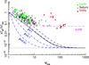Fig. 1 Electron-ion temperature ratio expected for minimum electron-heating (solid black line, Eq. (13)), for the case of adiabatic heating of the electrons (dashed black line, Eq. (22)), and for magnetised plasmas with β = 0.01,0.1,1 (blue dashed line, Eq 31). In addition the expected ratio is shown if on top of various thermodynamic effects there is energy exchange between the electrons and ions at the level of 5% (magenta dashed line, Eq. (A.7)). For the calculation here it is assumed that the plasma consists of electrons, protons, and fully ionised helium, and the ion temperature is the average temperature of abundance weighted temperature of the protons and helium ions. The data points are from the compilation by Ghavamian et al. (2013), and represent measured values of the electron-ion temperature ratio behind the Earth bowshock (green circles, original data from Schwartz et al. 1988), Saturn’s bowshock as measured by the Cassini spacecraft (X-shaped symbols, Masters et al. 2013) and supernova remnants (red, solid squares, van Adelsberg et al. 2008). Note that for the supernova remnants the Mach numbers are not measured, but instead the estimated shock velocity has been divided by assumed interstellar sound speed of 11 km s-1 (Ghavamian et al. 2013).

2.2. Adiabatic heating of the electrons

A result of Eq. (11) is that for low Mach numbers (M_s ≲ 60) the electron temperature is almost isothermal across the shock. This would mean that the entropy of the electron gas is decreasing, although the total entropy of the plasma is increasing. The question is whether this is physically a valid result or not. In a closed system the entropy should aways be constant or increase, but in this case the electrons are not an isolated system. It is, therefore, more likely that the electrons are at least adiabatically heated due to the compression caused by ions. To take adiabatic electron heating into account we first have to calculate the work done by the ions on the electrons for adiabatic compression.

We start with modifying Eq. (9) to include an additional enthalpy-flux term, q_e,ad, which is the excess enthalpy flux needed to adiabatically compress the electrons: 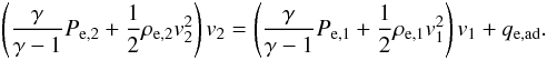$\begin{array}{ccc}\left(\frac{\mathit{\gamma }}{\mathit{\gamma }\mathrm{-}\mathrm{1}}{\mathit{P}}_{\mathrm{e}\mathit{,}\mathrm{2}}\mathrm{+}\frac{\mathrm{1}}{\mathrm{2}}{\mathit{\rho }}_{\mathrm{e}\mathit{,}\mathrm{2}}{\mathit{v}}_{\mathrm{2}}^{\mathrm{2}}\right){\mathit{v}}_{\mathrm{2}}\mathrm{=}\left(\frac{\mathit{\gamma }}{\mathit{\gamma }\mathrm{-}\mathrm{1}}{\mathit{P}}_{\mathrm{e}\mathit{,}\mathrm{1}}\mathrm{+}\frac{\mathrm{1}}{\mathrm{2}}{\mathit{\rho }}_{\mathrm{e}\mathit{,}\mathrm{1}}{\mathit{v}}_{\mathrm{1}}^{\mathrm{2}}\right){\mathit{v}}_{\mathrm{1}}\mathrm{+}{\mathit{q}}_{\mathrm{e}\mathit{,}\mathrm{ad}}\mathit{.}& & \end{array}$(15)For adiabatic compression the relation between pre- and post-shock electron pressures and temperatures is 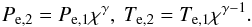$\begin{array}{ccc}{\mathit{P}}_{\mathrm{e}\mathit{,}\mathrm{2}}\mathrm{=}{\mathit{P}}_{\mathrm{e}\mathit{,}\mathrm{1}}{\mathit{\chi }}^{\mathit{\gamma }}\mathit{,}{\mathit{T}}_{\mathrm{e}\mathit{,}\mathrm{2}}\mathrm{=}{\mathit{T}}_{\mathrm{e}\mathit{,}\mathrm{1}}{\mathit{\chi }}^{\mathit{\gamma }\mathrm{-}\mathrm{1}}\mathit{.}& & \end{array}$(16)If one strictly wants to observe Eq. (16) one obtains, from inserting Eq. (16) in Eq. (15) 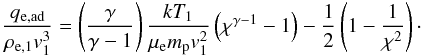$\begin{array}{ccc}\frac{{\mathit{q}}_{\mathrm{e}\mathit{,}\mathrm{ad}}}{{\mathit{\rho }}_{\mathrm{e}\mathit{,}\mathrm{1}}{\mathit{v}}_{\mathrm{1}}^{\mathrm{3}}}\mathrm{=}\left(\frac{\mathit{\gamma }}{\mathit{\gamma }\mathrm{-}\mathrm{1}}\right)\frac{\mathit{k}{\mathit{T}}_{\mathrm{1}}}{{\mathit{\mu }}_{\mathrm{e}}{\mathit{m}}_{\mathrm{p}}{\mathit{v}}_{\mathrm{1}}^{\mathrm{2}}}\mathrm{(}{\mathit{\chi }}^{\mathit{\gamma }\mathrm{-}\mathrm{1}}\mathrm{-}{\mathrm{1}}^{\mathrm{)}}\mathrm{-}\frac{\mathrm{1}}{\mathrm{2}}\left(\mathrm{1}\mathrm{-}\frac{\mathrm{1}}{{\mathit{\chi }}^{\mathrm{2}}}\right)\mathrm{·}& & \end{array}$(17)This expression for q_e,ad consists of two terms; the first term ensures that the temperature will be proportional to χ^γ−1, whereas the second term suppresses the heating due to the kinetic energy flux of the electrons themselves. The problem with this equation is exactly this second term, because this term counteracts for high Mach numbers (i.e. M_s ≳ 60, as derived in Sect. 2.1) the heating of electrons from thermalising their own kinetic energy. What is needed, therefore, is an expression for q_e,ad that enforces adiabatic heating at low Mach numbers (M_s ≲ 10) through the work done by the ions, whereas for M_s ≳ 60 the electron kinetic energy flux is more than sufficient to heat the electrons to temperatures beyond adiabatic compression. These two conditions are met if one omits the second term on the right hand side of Eq. (17), i.e. the term that suppresses thermalisation of the electron kinetic energy. Hence, the expression for the work done by the ions on the electrons becomes $\begin{array}{ccc}\frac{{\mathit{q}}_{\mathrm{e}\mathit{,}\mathrm{ad}}}{{\mathit{\rho }}_{\mathrm{e}\mathit{,}\mathrm{1}}{\mathit{v}}_{\mathrm{1}}^{\mathrm{3}}}\mathrm{=}\left(\frac{\mathit{\gamma }}{\mathit{\gamma }\mathrm{-}\mathrm{1}}\right)\frac{\mathit{k}{\mathit{T}}_{\mathrm{1}}}{{\mathit{\mu }}_{\mathrm{e}}{\mathit{m}}_{\mathrm{p}}{\mathit{v}}_{\mathrm{1}}^{\mathrm{2}}}\mathrm{(}{\mathit{\chi }}^{\mathit{\gamma }\mathrm{-}\mathrm{1}}\mathrm{-}{\mathrm{1}}^{\mathrm{)}}\mathit{.}& & \end{array}$(18)This expression and it is use in Eq. (15) seems a natural choice, but is not completely from first principles. It assumes implicitly that the ions will always first establish the shock, thereby compressing ad adiabatically heating the electrons, and that subsequently the electron kinetic energy is thermalised. In reality the electrons may be less passive when it comes to compressing the plasma, and part of the energy needed for adiabatic heating is provided by the electrons themselves. However, this is a concern only for intermediate Mach number shocks, since at Mach numbers below M_s ≲ 10 the electrons do not provide sufficient kinetic energy flux, whereas for M_s ≳ 60 the kinetic energy of the electrons is more than enough to provide heating much beyond adiabatic heating, and the effect of introducing q_e,ad is neglible.

Adopting Eq. (18) for the enthalpy-flux exchange between ions and electrons the expression for the downstream electron temperature becomes $\begin{array}{ccc}\frac{\mathit{k}{\mathit{T}}_{\mathrm{e}\mathit{,}\mathrm{2}}}{{\mathit{\mu }}_{\mathrm{e}}{\mathit{m}}_{\mathrm{p}}{\mathit{v}}_{\mathrm{1}}^{\mathrm{2}}}\mathrm{=}\frac{\mathit{k}{\mathit{T}}_{\mathrm{e}\mathit{,}\mathrm{1}}}{{\mathit{\mu }}_{\mathrm{e}}{\mathit{m}}_{\mathrm{p}}{\mathit{v}}_{\mathrm{1}}^{\mathrm{2}}}{\mathit{\chi }}^{\mathit{\gamma }\mathrm{-}\mathrm{1}}\mathrm{+}\frac{\mathrm{1}}{\mathrm{2}}\left(\frac{\mathit{\gamma }\mathrm{-}\mathrm{1}}{\mathit{\gamma }}\right)\left(\mathrm{1}\mathrm{-}\frac{\mathrm{1}}{{\mathit{\chi }}^{\mathrm{2}}}\right)\mathrm{=}\frac{\mathrm{1}}{\mathit{\gamma }{\mathit{M}}_{\mathrm{s}}^{\mathrm{2}}}\left(\frac{\mathit{\mu }}{{\mathit{\mu }}_{\mathrm{e}}}\right){\mathit{\chi }}^{\mathit{\gamma }\mathrm{-}\mathrm{1}}\mathrm{+}\frac{\mathrm{1}}{\mathrm{2}}\left(\frac{\mathit{\gamma }\mathrm{-}\mathrm{1}}{\mathit{\gamma }}\right)\left(\mathrm{1}\mathrm{-}\frac{\mathrm{1}}{{\mathit{\chi }}^{\mathrm{2}}}\right)\mathrm{·}& & \end{array}$(19)Note that we made use of Eq. (8) in order to introduce the sonic Mach number. One recognises in this equation again the two sources of heating, with the first term being associated with adiabatic heating by the ions and the second term being associated with the thermalisation of the electron kinetic energy, which asymptotically approaches Eq. (2).

We illustrate the effects of adiabatic heating and thermalisation of the kinetic energy of the electrons in Fig. 2, which shows the ratio of downstream over upstream electron temperatures as given by Eq. (19) and comparing it to the result of Eq. (10) and adiabatic heating only (i.e. if one would use q_e,ad as given in Eq. (17)). It shows that at low Mach numbers Eq. (19) results in only adiabatic heating, whereas for very high Mach number Eq. (19) asymptotically approaches Eq. (10).

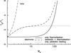Fig. 2 Ratio of the electron temperature upstream and downstream (Te,2/Ti,2), resulting from different assumptions. The dashed line corresponds to Eq. (19) (adiabatic heating and thermalisation), the solid line corresponds to Eq. (10). For illustrative purposes we also show the effect of adiabatic compression alone (dotted line) and the upstream and upstream temperature ratios for ions (dot-dashed line).

The work done on the electrons will be at the cost of the heating of the ions. We, therefore, have to subtract q_e,ad (Eq. (18)) from the ion-enthalpy flux: $\begin{array}{ccc}\left(\frac{\mathit{\gamma }}{\mathit{\gamma }\mathrm{-}\mathrm{1}}{\mathit{P}}_{\mathrm{i}\mathit{,}\mathrm{2}}\mathrm{+}\frac{\mathrm{1}}{\mathrm{2}}{\mathit{\rho }}_{\mathrm{i}\mathit{,}\mathrm{2}}{\mathit{v}}_{\mathrm{2}}^{\mathrm{2}}\right){\mathit{v}}_{\mathrm{2}}\mathrm{=}& \left(\frac{\mathit{\gamma }}{\mathit{\gamma }\mathrm{-}\mathrm{1}}{\mathit{P}}_{\mathrm{i}\mathit{,}\mathrm{1}}\mathrm{+}\frac{\mathrm{1}}{\mathrm{2}}{\mathit{\rho }}_{\mathrm{i}\mathit{,}\mathrm{1}}{\mathit{v}}_{\mathrm{1}}^{\mathrm{2}}\right){\mathit{v}}_{\mathrm{1}}\mathrm{-}{\mathit{q}}_{\mathrm{e}\mathit{,}\mathrm{ad}}\mathit{.}& \end{array}$(20)Equations (20) and (15) added together just express that enthalpy-flux across the shock is conserved (Eq. (5)). This equation results in the following expression for the ion temperature: $\begin{array}{ccc}\frac{\mathit{k}{\mathit{T}}_{\mathrm{i}\mathit{,}\mathrm{2}}}{{\mathit{\mu }}_{\mathrm{i}}{\mathit{m}}_{\mathrm{p}}{\mathit{v}}_{\mathrm{1}}^{\mathrm{2}}}& \mathrm{=}& \frac{\mathit{k}{\mathit{T}}_{\mathrm{i}\mathit{,}\mathrm{1}}}{{\mathit{\mu }}_{\mathrm{i}}{\mathit{m}}_{\mathrm{p}}{\mathit{v}}_{\mathrm{1}}^{\mathrm{2}}}\left[\mathrm{1}\mathrm{-}\left(\frac{{\mathit{n}}_{\mathrm{e}\mathit{,}\mathrm{1}}}{{\mathit{n}}_{\mathrm{i}\mathit{,}\mathrm{1}}}\right)\mathrm{(}{\mathit{\chi }}^{\mathit{\gamma }\mathrm{-}\mathrm{1}}\mathrm{-}{\mathrm{1}}^{\mathrm{)}}\right]\mathrm{+}\frac{\mathrm{1}}{\mathrm{2}}\left(\frac{\mathit{\gamma }\mathrm{-}\mathrm{1}}{\mathit{\gamma }}\right)\left(\mathrm{1}\mathrm{-}\frac{\mathrm{1}}{{\mathit{\chi }}^{\mathrm{2}}}\right)\\ & \mathrm{=}& \frac{\mathrm{1}}{\mathit{\gamma }{\mathit{M}}_{\mathrm{s}}^{\mathrm{2}}}\left(\frac{\mathit{\mu }}{{\mathit{\mu }}_{\mathrm{i}}}\right)\left[\mathrm{1}\mathrm{-}\left(\frac{{\mathit{n}}_{\mathrm{e}\mathit{,}\mathrm{1}}}{{\mathit{n}}_{\mathrm{i}\mathit{,}\mathrm{1}}}\right)\mathrm{(}{\mathit{\chi }}^{\mathit{\gamma }\mathrm{-}\mathrm{1}}\mathrm{-}{\mathrm{1}}^{\mathrm{)}}\right]\mathrm{+}\frac{\mathrm{1}}{\mathrm{2}}\left(\frac{\mathit{\gamma }\mathrm{-}\mathrm{1}}{\mathit{\gamma }}\right)\left(\mathrm{1}\mathrm{-}\frac{\mathrm{1}}{{\mathit{\chi }}^{\mathrm{2}}}\right)\mathrm{·}\end{array}$(21)As a result the post-shock, electron-ion temperature ratio will be $\begin{array}{ccc}\frac{{\mathit{T}}_{\mathrm{e}\mathit{,}\mathrm{2}}}{{\mathit{T}}_{\mathrm{i}\mathit{,}\mathrm{2}}}\mathrm{=}\left(\frac{{\mathit{\mu }}_{\mathrm{e}}}{{\mathit{\mu }}_{\mathrm{i}}}\right)\frac{\mathrm{2}\left(\frac{\mathit{\mu }}{{\mathit{\mu }}_{\mathrm{e}}}\right){\mathit{\chi }}^{\mathit{\gamma }\mathrm{+}\mathrm{1}}\mathrm{+}{\mathit{M}}_{\mathrm{s}}^{\mathrm{2}}\left(\mathit{\gamma }\mathrm{-}\mathrm{1}\right)\mathrm{(}{\mathit{\chi }}^{\mathrm{2}}\mathrm{-}\mathrm{1}\mathrm{)}}{\mathrm{2}\left(\frac{\mathit{\mu }}{{\mathit{\mu }}_{\mathrm{i}}}\right){\mathit{\chi }}^{\mathrm{2}}\left[\mathrm{1}\mathrm{-}\left(\frac{{\mathit{n}}_{\mathrm{e}\mathit{,}\mathrm{1}}}{{\mathit{n}}_{\mathrm{i}\mathit{,}\mathrm{1}}}\right)\left({\mathit{\chi }}^{\mathit{\gamma }\mathrm{-}\mathrm{1}}\mathrm{-}\mathrm{1}\right)\right]\mathrm{+}{\mathit{M}}_{\mathrm{s}}^{\mathrm{2}}\left(\mathit{\gamma }\mathrm{-}\mathrm{1}\right)\mathrm{(}{\mathit{\chi }}^{\mathrm{2}}\mathrm{-}\mathrm{1}\mathrm{)}}\mathrm{·}& & \end{array}$(22)Comparing this equation with Eq. (13) we see many similarities. The correctional factor in the denominator, given in square brackets, is small, as only a small fraction of the ion-enthalpy needs to be used to adiabatically heat the electrons. In the numerator we see that the factor χ² has been replaced by χ^{γ + 1}. For very high Mach numbers, roughly M_s> 60 as derived in the previous section, the second term in the numerator becomes dominant and the electrons are heated beyond adiabatic heating. However, the overall scaling of electron-ion temperature ratio is similar to Eq. (13), namely ${\mathit{T}}_{\mathrm{e}\mathit{,}\mathrm{2}}\mathit{/}{\mathit{T}}_{\mathrm{i}\mathit{,}\mathrm{2}}\mathrm{\propto }\mathrm{1}\mathit{/}{\mathit{M}}_{\mathrm{s}}^{\mathrm{2}}$ for 5 ≲ <M_s ≲ 60, as can be seen in Fig. 1 (dashed black line). The temperature ratio is, however, larger than given by Eq. (13) (solid black line).

2.3. The electron-ion temperature ratio in magnetised shocks

In the previous subsections we have ignored the effects of magnetic fields. It is likely that the magnetic field and plasma waves play an important role in the heating of the electrons and ions in collisionless shocks. However, here we focus on the importance of the shock thermodynamics on the expected electron-ion temperature ratio. From a purely thermodynamic point of view the magnetic field is important as it results in an additional pressure term, and the compression of the magnetic field requires additional work to be done on the plasma. The free energy-flux available for doing work on the magnetised plasma will come mainly from the ion kinetic energy, as this is the largest reservoir of free energy. This suggests that the downstream ion temperature will be lower for a given shock velocity if the shock is strongly magnetised. As we will see below this is indeed the case as one compares magnetised shocks with unmagnetised shocks for a given sonic Mach number, M_s. However, for a magnetised shock the relevant Mach number is the magnetosonic Mach number, M_ms. To illustrate the effects of the magnetic field strength on the electron-ion temperature ratio we calculate here the thermodynamic effects of a magnetic field that is align strictly perpendicular to the shock normal (B_⊥ = B).

We parameterise the effects of the magnetic field using the plasma-beta parameter $\begin{array}{ccc}\mathit{\beta }\mathrm{\equiv }\frac{{\mathit{P}}_{\mathrm{T}\mathit{,}\mathrm{1}}}{{\mathit{P}}_{\mathrm{B}\mathit{,}\mathrm{1}}}\mathrm{=}\frac{\mathrm{8}\mathit{\pi }\mathrm{(}{\mathit{n}}_{\mathrm{i}\mathit{,}\mathrm{1}}\mathrm{+}{\mathit{n}}_{\mathrm{e}\mathit{,}\mathrm{1}}\mathrm{)}\mathit{k}{\mathit{T}}_{\mathrm{1}}}{{\mathit{B}}_{\mathrm{1}}^{\mathrm{2}}}\mathit{,}& & \end{array}$(23)with P_T,1 representing the total upstream, thermal pressure (electrons plus ions) and P_B,1 the upstream magnetic pressure. It is assumed here that upstream the electron and ion temperatures are equal (kT_e,1 = kT_i,1 = kT₁). The ratio of the shock velocity to the Alfvén velocity, V_A = B₁/$\sqrt{\mathrm{4}\mathit{\pi }{\mathit{\rho }}_{\mathrm{1}}}$, is the Alfvén Mach number, M_A = V_s/V_A. Note that the relation between Alfvén Mach number and sonic Mach number is given by the equation $\begin{array}{ccc}{\mathit{M}}_{\mathrm{s}}^{\mathrm{2}}\mathrm{=}\frac{\mathrm{2}}{\mathit{\gamma \beta }}{\mathit{M}}_{\mathrm{A}}^{\mathrm{2}}\mathrm{·}& & \end{array}$(24)These relations are useful, because the thermal pressure component of the downstream plasma is best parametrised by the sonic Mach number, whereas the shock compression ratio is mainly determined by the magnetosonic Mach number defined as 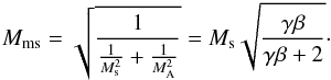$\begin{array}{ccc}{\mathit{M}}_{\mathrm{ms}}\mathrm{=}\sqrt{\frac{\mathrm{1}}{\frac{\mathrm{1}}{{\mathit{M}}_{\mathrm{s}}^{\mathrm{2}}}\mathrm{+}\frac{\mathrm{1}}{{\mathit{M}}_{\mathrm{A}}^{\mathrm{2}}}}}\mathrm{=}{\mathit{M}}_{\mathrm{s}}\sqrt{\frac{\mathit{\gamma \beta }}{\mathit{\gamma \beta }\mathrm{+}\mathrm{2}}}\mathrm{·}& & \end{array}$(25)The shock compression ratios for perpendicular, magnetised shocks is given by Tidman & Krall (1971) for γ = 5/3, and can be expressed in the dimensionless numbers β and M_s as 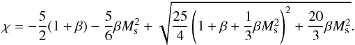$\begin{array}{ccc}\mathit{\chi }\mathrm{=}\mathrm{-}\frac{\mathrm{5}}{\mathrm{2}}\mathrm{(}\mathrm{1}\mathrm{+}\mathit{\beta }\mathrm{)}\mathrm{-}\frac{\mathrm{5}}{\mathrm{6}}\mathit{\beta }{\mathit{M}}_{\mathrm{s}}^{\mathrm{2}}\mathrm{+}\sqrt{\frac{\mathrm{25}}{\mathrm{4}}{\left(\mathrm{1}\mathrm{+}\mathit{\beta }\mathrm{+}\frac{\mathrm{1}}{\mathrm{3}}\mathit{\beta }{\mathit{M}}_{\mathrm{s}}^{\mathrm{2}}\right)}^{\mathrm{2}}\mathrm{+}\frac{\mathrm{20}}{\mathrm{3}}\mathit{\beta }{\mathit{M}}_{\mathrm{s}}^{\mathrm{2}}}\mathit{.}& & \end{array}$(26)There are two effects of magnetic fields on the electron-ion temperature ratio: 1) for β ≪ 1 the sonic Mach number is much larger than the magnetosonic Mach number M_s ≫ M_ms, as a consequence the electron-ion temperature ratio is expected to be lower given Eq. (13) and/or Eq. (22); 2) the kinetic energy of the ions will be partially used to do work on the magnetic field in order to compress it. In analogy with Eq. (18) we introduce here a parameter q_B, which is the enthalpy flux necessary to compress the magnetic field: 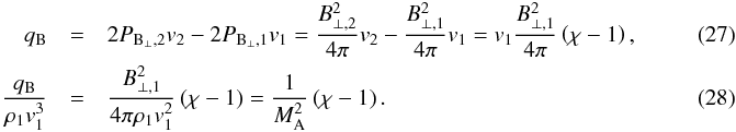$\begin{array}{ccc}{\mathit{q}}_{\mathrm{B}}& \mathrm{=}& \mathrm{2}{\mathit{P}}_{{\mathrm{B}}_{\mathrm{\perp }}\mathit{,}\mathrm{2}}{\mathit{v}}_{\mathrm{2}}\mathrm{-}\mathrm{2}{\mathit{P}}_{{\mathrm{B}}_{\mathrm{\perp }}\mathit{,}\mathrm{1}}{\mathit{v}}_{\mathrm{1}}\mathrm{=}\frac{{\mathit{B}}_{\mathrm{\perp }\mathit{,}\mathrm{2}}^{\mathrm{2}}}{\mathrm{4}\mathit{\pi }}{\mathit{v}}_{\mathrm{2}}\mathrm{-}\frac{{\mathit{B}}_{\mathrm{\perp }\mathit{,}\mathrm{1}}^{\mathrm{2}}}{\mathrm{4}\mathit{\pi }}{\mathit{v}}_{\mathrm{1}}\mathrm{=}{\mathit{v}}_{\mathrm{1}}\frac{{\mathit{B}}_{\mathrm{\perp }\mathit{,}\mathrm{1}}^{\mathrm{2}}}{\mathrm{4}\mathit{\pi }}\left(\mathit{\chi }\mathrm{-}\mathrm{1}\right)\mathit{,}\\ \frac{{\mathit{q}}_{\mathrm{B}}}{{\mathit{\rho }}_{\mathrm{1}}{\mathit{v}}_{\mathrm{1}}^{\mathrm{3}}}& \mathrm{=}& \frac{{\mathit{B}}_{\mathrm{\perp }\mathit{,}\mathrm{1}}^{\mathrm{2}}}{\mathrm{4}\mathit{\pi }{\mathit{\rho }}_{\mathrm{1}}{\mathit{v}}_{\mathrm{1}}^{\mathrm{2}}}\left(\mathit{\chi }\mathrm{-}\mathrm{1}\right)\mathrm{=}\frac{\mathrm{1}}{{\mathit{M}}_{\mathrm{A}}^{\mathrm{2}}}\left(\mathit{\chi }\mathrm{-}\mathrm{1}\right)\mathit{.}\end{array}$We now proceed as before by calculating the ion temperature from the enthalpy-flux equation for the ions only: 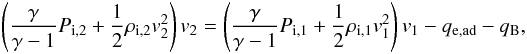$\begin{array}{ccc}\left(\frac{\mathit{\gamma }}{\mathit{\gamma }\mathrm{-}\mathrm{1}}{\mathit{P}}_{\mathrm{i}\mathit{,}\mathrm{2}}\mathrm{+}\frac{\mathrm{1}}{\mathrm{2}}{\mathit{\rho }}_{\mathrm{i}\mathit{,}\mathrm{2}}{\mathit{v}}_{\mathrm{2}}^{\mathrm{2}}\right){\mathit{v}}_{\mathrm{2}}\mathrm{=}\left(\frac{\mathit{\gamma }}{\mathit{\gamma }\mathrm{-}\mathrm{1}}{\mathit{P}}_{\mathrm{i}\mathit{,}\mathrm{1}}\mathrm{+}\frac{\mathrm{1}}{\mathrm{2}}{\mathit{\rho }}_{\mathrm{i}\mathit{,}\mathrm{1}}{\mathit{v}}_{\mathrm{1}}^{\mathrm{2}}\right){\mathit{v}}_{\mathrm{1}}\mathrm{-}{\mathit{q}}_{\mathrm{e}\mathit{,}\mathrm{ad}}\mathrm{-}{\mathit{q}}_{\mathrm{B}}\mathit{,}& & \end{array}$(29)which can be worked out to give the following downstream ion temperature $\begin{array}{ccc}\frac{\mathit{k}{\mathit{T}}_{\mathrm{i}\mathit{,}\mathrm{2}}}{{\mathit{\mu }}_{\mathrm{i}}{\mathit{m}}_{\mathrm{p}}{\mathit{v}}_{\mathrm{1}}^{\mathrm{2}}}& \mathrm{=}& \frac{\mathit{k}{\mathit{T}}_{\mathrm{i}\mathit{,}\mathrm{1}}}{{\mathit{\mu }}_{\mathrm{i}}{\mathit{m}}_{\mathrm{p}}{\mathit{v}}_{\mathrm{1}}^{\mathrm{2}}}\left[\mathrm{1}\mathrm{-}\left(\frac{{\mathit{n}}_{\mathrm{e}\mathit{,}\mathrm{1}}}{{\mathit{n}}_{\mathrm{i}\mathit{,}\mathrm{1}}}\right)\left(\frac{{\mathit{\mu }}_{\mathrm{e}}}{{\mathit{\mu }}_{\mathrm{i}}}\right)\mathrm{(}{\mathit{\chi }}^{\mathit{\gamma }\mathrm{-}\mathrm{1}}\mathrm{-}{\mathrm{1}}^{\mathrm{)}}\right]\mathrm{+}\frac{\mathrm{1}}{\mathrm{2}}\left(\frac{\mathit{\gamma }\mathrm{-}\mathrm{1}}{\mathit{\gamma }}\right)\left(\mathrm{1}\mathrm{-}\frac{\mathrm{1}}{{\mathit{\chi }}^{\mathrm{2}}}\right)\mathrm{-}\frac{\mathrm{1}}{{\mathit{M}}_{\mathrm{A}}^{\mathrm{2}}}\left(\frac{{\mathit{\rho }}_{\mathrm{1}}}{{\mathit{\rho }}_{\mathrm{i}\mathit{,}\mathrm{1}}}\right)\left(\frac{\mathit{\gamma }\mathrm{-}\mathrm{1}}{\mathit{\gamma }}\right)\left(\mathit{\chi }\mathrm{-}\mathrm{1}\right)\mathit{,}\\ & \mathrm{=}& \frac{\mathrm{1}}{\mathit{\gamma }{\mathit{M}}_{\mathrm{s}}^{\mathrm{2}}}\left(\frac{\mathit{\mu }}{{\mathit{\mu }}_{\mathrm{i}}}\right)\left[\mathrm{1}\mathrm{-}\left(\frac{{\mathit{n}}_{\mathrm{e}\mathit{,}\mathrm{1}}}{{\mathit{n}}_{\mathrm{i}\mathit{,}\mathrm{1}}}\right)\left(\frac{{\mathit{\mu }}_{\mathrm{e}}}{{\mathit{\mu }}_{\mathrm{i}}}\right)\mathrm{(}{\mathit{\chi }}^{\mathit{\gamma }\mathrm{-}\mathrm{1}}\mathrm{-}{\mathrm{1}}^{\mathrm{)}}\right]\mathrm{+}\frac{\mathrm{1}}{\mathrm{2}}\left(\frac{\mathit{\gamma }\mathrm{-}\mathrm{1}}{\mathit{\gamma }}\right)\left(\mathrm{1}\mathrm{-}\frac{\mathrm{1}}{{\mathit{\chi }}^{\mathrm{2}}}\right)\mathrm{-}\frac{\mathrm{2}}{\mathit{\beta \gamma }{\mathit{M}}_{\mathrm{s}}^{\mathrm{2}}}\left(\mathrm{1}\mathrm{+}\frac{{\mathit{n}}_{\mathrm{e}\mathit{,}\mathrm{1}}}{{\mathit{n}}_{\mathrm{i}\mathit{,}\mathrm{1}}}\frac{{\mathit{\mu }}_{\mathrm{e}}}{{\mathit{\mu }}_{\mathrm{i}}}\right)\left(\frac{\mathit{\gamma }\mathrm{-}\mathrm{1}}{\mathit{\gamma }}\right)\left(\mathit{\chi }\mathrm{-}\mathrm{1}\right)\mathit{,}\end{array}$(30)where we have made use of Eq. (24), in order to make M_s and β the primary shock parameters for magnetised shocks. The factor in square brackets comes from the work done to adiabatically heat the electrons (Sect. 2.2). If we only assume enthalpy-flux conservation for the electrons, this factor can be omitted. The factor (ρ/ρ_i) is very close to one.

We can calculate the electron-ion temperature ratio by combining Eq. (29) with Eq. (19), which results in $\begin{array}{ccc}\frac{{\mathit{T}}_{\mathrm{e}\mathit{,}\mathrm{2}}}{{\mathit{T}}_{\mathrm{i}\mathit{,}\mathrm{2}}}\mathrm{=}& & \left(\frac{{\mathit{\mu }}_{\mathrm{e}}}{{\mathit{\mu }}_{\mathrm{i}}}\right)\frac{\mathrm{2}\left(\frac{\mathit{\mu }}{{\mathit{\mu }}_{\mathrm{e}}}\right){\mathit{\chi }}^{\mathit{\gamma }\mathrm{+}\mathrm{1}}\mathrm{+}{\mathit{M}}_{\mathrm{s}}^{\mathrm{2}}\left(\mathit{\gamma }\mathrm{-}\mathrm{1}\right)\mathrm{(}{\mathit{\chi }}^{\mathrm{2}}\mathrm{-}\mathrm{1}\mathrm{)}}{\mathrm{2}\left(\frac{\mathit{\mu }}{{\mathit{\mu }}_{\mathrm{i}}}\right){\mathit{\chi }}^{\mathrm{2}}\left[\mathrm{1}\mathrm{-}\left(\frac{{\mathit{n}}_{\mathrm{e}\mathit{,}\mathrm{1}}}{{\mathit{n}}_{\mathrm{i}\mathit{,}\mathrm{1}}}\right)\left(\frac{{\mathit{\mu }}_{\mathrm{e}}}{{\mathit{\mu }}_{\mathrm{i}}}\right)\left({\mathit{\chi }}^{\mathit{\gamma }\mathrm{-}\mathrm{1}}\mathrm{-}\mathrm{1}\right)\right]\mathrm{+}{\mathit{M}}_{\mathrm{s}}^{\mathrm{2}}\left(\mathit{\gamma }\mathrm{-}\mathrm{1}\right)\mathrm{(}{\mathit{\chi }}^{\mathrm{2}}\mathrm{-}\mathrm{1}\mathrm{)}\mathrm{-}\frac{\mathrm{4}}{\mathit{\beta \gamma }}\left(\mathrm{1}\mathrm{+}\frac{{\mathit{n}}_{\mathrm{e}\mathit{,}\mathrm{1}}}{{\mathit{n}}_{\mathrm{i}\mathit{,}\mathrm{1}}}\frac{{\mathit{\mu }}_{\mathrm{e}}}{{\mathit{\mu }}_{\mathrm{i}}}\right)\left(\mathit{\gamma }\mathrm{-}\mathrm{1}\right){\mathit{\chi }}^{\mathrm{2}}\left(\mathit{\chi }\mathrm{-}\mathrm{1}\right)}\mathrm{·}\end{array}$(31)The dashed blue lines in Fig. 1 shows the derived electron-ion temperature ratio for various values of β. Note that for β = 1 the predicted ratio is close to an unmagnetised shock without adiabatic heating.

For completeness’ sake we also give here the electrons the electron-ion temperature ratio for a magnetised shock without adiabatic heating: 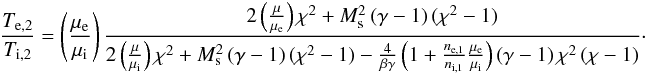$\begin{array}{ccc}\frac{{\mathit{T}}_{\mathrm{e}\mathit{,}\mathrm{2}}}{{\mathit{T}}_{\mathrm{i}\mathit{,}\mathrm{2}}}\mathrm{=}\left(\frac{{\mathit{\mu }}_{\mathrm{e}}}{{\mathit{\mu }}_{\mathrm{i}}}\right)\frac{\mathrm{2}\left(\frac{\mathit{\mu }}{{\mathit{\mu }}_{\mathrm{e}}}\right){\mathit{\chi }}^{\mathrm{2}}\mathrm{+}{\mathit{M}}_{\mathrm{s}}^{\mathrm{2}}\left(\mathit{\gamma }\mathrm{-}\mathrm{1}\right)\mathrm{(}{\mathit{\chi }}^{\mathrm{2}}\mathrm{-}\mathrm{1}\mathrm{)}}{\mathrm{2}\left(\frac{\mathit{\mu }}{{\mathit{\mu }}_{\mathrm{i}}}\right){\mathit{\chi }}^{\mathrm{2}}\mathrm{+}{\mathit{M}}_{\mathrm{s}}^{\mathrm{2}}\left(\mathit{\gamma }\mathrm{-}\mathrm{1}\right)\mathrm{(}{\mathit{\chi }}^{\mathrm{2}}\mathrm{-}\mathrm{1}\mathrm{)}\mathrm{-}\frac{\mathrm{4}}{\mathit{\beta \gamma }}\left(\mathrm{1}\mathrm{+}\frac{{\mathit{n}}_{\mathrm{e}\mathit{,}\mathrm{1}}}{{\mathit{n}}_{\mathrm{i}\mathit{,}\mathrm{1}}}\frac{{\mathit{\mu }}_{\mathrm{e}}}{{\mathit{\mu }}_{\mathrm{i}}}\right)\left(\mathit{\gamma }\mathrm{-}\mathrm{1}\right){\mathit{\chi }}^{\mathrm{2}}\left(\mathit{\chi }\mathrm{-}\mathrm{1}\right)}\mathrm{·}& & \end{array}$(32)

2.4. How much non-adiabatic heat exchange is there between ions and electrons?

In the preceding subsections we have approached the expected electron-ion temperature ratio from the point of view of the available enthalpy of the electron and ion components separately, but allowing for adiabatic heating of the electrons (Sect. 2.2) and the fact that for magnetised plasma’s work has to be done by mostly the ions to compress the magnetic field (Sect. 2.3).

However, collisionless shock heating is a complex process, and the microphysics of the heating process of both the ions and electrons is not well understood. In the Appendix (Sect. A) we show how one can quantify the additional thermal energy that the electrons pick-up from ions. This is done by introducing an electron-ion heat exhange parameter ξ. A value of ξ = 50% corresponds to a fully equilibrated plasma, whereas ξ = 0 gives the same result as Eq. (31).

Figure 1 shows the electron/ion temperature ratio for ξ = 5%, which seems to approximately describe the levelling off of the electron-ion temperature ratio seen in the Earth bow shock for magnetosonic Mach numbers above ~20. However, more data are needed to see whether this is a general trend, as there are not that many data points above M_s = 10. The supernova remnant shocks have generally higher Mach numbers, but for them the actually Mach numbers are poorly constraint as we discuss below.

3. Discussion

The relation that we derived for the electron-ion temperature ratio is simple and based on the assumption that all particle species observe the same density jump, but that the electron and ion enthalpy fluxes are preserved separately. The only additional heating of the electrons that we allow for (Sect. 2.2) is due to heating by adiabatic compression. In this framework, the potential role of the magnetic field (Sect. 2.3) is passive: magnetised shocks (β< 1) have a lower upstream electron/ion pressure for a given overall pressure. Or to put it differently, the sonic Mach number is higher for a given magnetosonic Mach number, as compared to plasmas with a larger plasma-beta. The electron/ion temperature ratio is in our explanation determined by the sonic Mach number and not by the magnetosonic Mach number.

In addition, we introduced enthalpy-flow exchange between ions and electrons using a dimensionless variable ξ, with (realistically) 0% ≤ ξ ≤ 50%, with ξ = 0 corresponding to full non-equilibration. We stress that this is an heuristic approach.

Comparing our relations with the measurements (Fig. 1) shows that the electron-ion temperature ratio predicted by the adiabatic heating case (Eq. (22)) seems to describe the measurements best for Mach numbers between 1 and ~10, whereas the the pure elastic scattering case (Eq. (13)) appears to form a firm lower limit to the measured temperature ratios. However, adiabatic heating of the electrons for magnetised plasma with β = 1 also seems to provide a lower limit to the measured electron-ion temperature ratio. Magnetisation seems to be a more likely explanation for the low electron/ion temperature ratios. For Mach numbers M_ms ≳ 10 the temperature ratio appears to asymptotically reach a value that is far above the relations as predicted by thermodynamic processes alone.

For a few data points relating to solar system shocks, the electrons appear to be hotter than the ions. These points cannot be explained by our simple model. It may hint at possible heating of the electrons upstream of the sub-shock, perhaps caused by ions reflected from the subshock (Cargill & Papadopoulos 1988). But it is not quite clear from the literature whether the measured temperature ratios are inconsistent with our relations given the unknown measurement errors, and systematic uncertainties.

The measured SNR temperature ratios seem to behave differently than the solar-system temperature ratios. As noted by Ghavamian et al. (2013), they do observe the relation ${\mathit{T}}_{\mathrm{e}}\mathit{/}{\mathit{T}}_{\mathrm{i}}\mathrm{\propto }{\mathit{M}}_{\mathrm{s}}^{-2}$, but the data points are shifted to higher Mach numbers as compared to the solar system measurements. But, as explained by Ghavamian et al. (2013), for SNRs the actual Mach number is not directly measured, but at best only the shock velocity is measured. The Mach numbers are then inferred by assuming that the local sound speed is 11 km s^-1. Assuming a higher local, upstream sound speed would shift the SNR temperature ratios closer to the solar-system values. This could either imply larger temperatures near supernova remnant shocks, but it could also mean that cosmic-ray precursors have pre-heated the plasma before entering the shock, as already emphasised by Ghavamian et al. (2013).

The effect of efficient cosmic-ray acceleration on the electron-ion temperature ratio can be estimated by using the relations between post-shock, fractional cosmic ray pressure downstream of the shock, w₂ = P_cr/P_tot, and adiabatic compression in the cosmic-ray precursor, as derived in Vink et al. (2010) and Vink & Yamazaki (2014). The basic assumptions in these papers are that the cosmic-ray precursor induces a pre-compression upstream of the shock χ_prec, resulting a in a lower Mach number at the actual gas shock (sub-shock) to ${\mathit{M}}_{\mathrm{s}\mathit{,}\mathrm{sub}}^{\mathrm{2}}\mathrm{=}{\mathit{M}}_{\mathrm{s}}^{\mathrm{2}}{\mathit{\chi }}_{\mathrm{prec}}^{\mathrm{-}\mathit{\gamma }}$. The relation between fractional cosmic-ray pressure w₂, precursor compression, and overall compression ratio, χ_tot was derived by Vink et al. (2010) to be 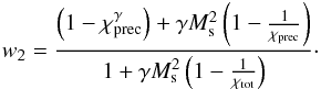$\begin{array}{ccc}{\mathit{w}}_{\mathrm{2}}\mathrm{=}\frac{\mathrm{(}\mathrm{1}\mathrm{-}{{\mathit{\chi }}_{\mathrm{prec}}^{\mathit{\gamma }}}^{\mathrm{)}}\mathrm{+}\mathit{\gamma }{\mathit{M}}_{\mathrm{s}}^{\mathrm{2}}\left(\mathrm{1}\mathrm{-}\frac{\mathrm{1}}{{\mathit{\chi }}_{\mathrm{prec}}}\right)}{\mathrm{1}\mathrm{+}\mathit{\gamma }{\mathit{M}}_{\mathrm{s}}^{\mathrm{2}}\left(\mathrm{1}\mathrm{-}\frac{\mathrm{1}}{{\mathit{\chi }}_{\mathrm{tot}}}\right)}\mathrm{·}& & \end{array}$(33)Using these relations, we can calculate the electron-ion temperature ratio by assuming that in the precursor ions and electrons are adiabatically heated to the same temperature and only at the sub-shock, with its reduced Mach number, the electrons and ions are shock heated to the temperature ratio given by Eq. (13). The effect of the cosmic-ray precursor on the electron-ion temperature ratio is shown in Fig. 3. Clearly the effects are modest, except for very high cosmic-ray acceleration efficiencies (w₂ ≳ 0.5). The effects could be larger if in the precursor also other, non-adiabatic, heating processes play a role.There is observational evidence, based on narrow line Hα emission, that the upstream plasma of young SNRs is indeed hotter than expected (Sollerman et al. 2003), perhaps as a result of heating in the cosmic-ray precursor. If the pre-heating of the neutral particles in the precursor is caused by charge exchange of the neutral particles with the heated ions in the precursor (Raymond et al. 2011; Blasi et al. 2012), then the neutral particles provide a measure of the temperature in the precursor at a distance l ≈ τ_cxv₁ from the sub-shock (with τ_cx the average time between charge exchanges). In contrast, the electron-ion temperature ratio is sensitive to the plasma temperature immediately upstream of the subshock. In fact, if by time we obtain sufficient faith in the relations proposed in this paper, we may use the measured electron-ion temperature ratio to infer the precursor temperature. However, preferential heating of electrons upstream of the shock, as perhaps indicated by some solar system shocks, may complicate the use of the downstream electron-ion temperature ratio as derived here.

Fig. 3 Electron-ion temperature ratio as a function of cosmic ray acceleration efficiency. The efficiency is defined here as the fraction w2 of post-shock cosmic-ray pressure (assumed here to be characterised by an adiabatic index of γcr = 1.5) to the overall pressure. The cosmic-ray efficiency is linked to the Mach number at the sub-shock, which has been affected by the compression of the plasma in the cosmic-ray precursor. See Vink et al. (2010) and Vink & Yamazaki (2014) for details.

Apart from the effects of cosmic-ray acceleration on the electron-ion temperature ratio, several other complications should be considered, which may, under certain circumstances, affect the electron temperatures, or may affect the interpretations of the measurements. One non-trivial issue concerns the definition of the electron temperature itself. It presumes that the electrons are thermalised, which for collisionless shocks may not always be the case. For example, Bykov & Uvarov (1999) find that under certain circumstances the energy distribution of the electrons is non-Maxwellian. On the other hand, if individual electrons are merely scattered elastically in the shock region, the electron velocity distribution may be isotropised, but the electrons are in that case almost mono-energetic, instead of having a Maxwellian distribution. In either case, further downstream of the shock the electrons may thermalise as a result of electron-electron Coulomb interactions. The timescale for electron-electron equilibration is relatively short (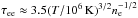${\mathit{\tau }}_{\mathrm{ee}}\mathrm{\approx }\mathrm{3.5}\mathrm{(}\mathit{T}\mathit{/}{\mathrm{10}}^{\mathrm{6}}\hspace{0.17em}\mathrm{K}{\mathrm{)}}^{\mathrm{3}\mathit{/}\mathrm{2}}{\mathit{n}}_{\mathrm{e}}^{\mathrm{-}\mathrm{1}\mathit{/}\mathrm{2}}$ months) compared to the electron-ion equilibration time scale (τ_ei ≈ 275(T/ 10⁶ K)^3/2 yr) (Spitzer 1965). For SNRs the measurable consequences may be limited, as the average electron temperatures are typically measured further downstream of the shocks. But for in situ measurements of temperatures downstream of heliospheric shocks, the electron temperature measured may not correspond to a well defined thermodynamic temperature. The shock jump conditions themselves are valid for any energy distribution of the particles, although the relation P = nkT cannot be blindly used, since a basic assumption of Eqs. (4) and (5) is that the pressure is isotropic. In essence the pressure term in Eq. (4) refers to the pressure along the shock normal, whereas in Eq. (5) the pressure refers to the isotropic pressure, or internal energy. A last caveat to discuss is that our ansatz for calculating the expected electron-ion temperature ratio assumes that the plasma upstream of the shock is fully ionised. Neutral particles entering the shock will ionise further downstream of the shock and result in a cold population of secondary electrons, which will slowly equilibrate with the primary electrons heated by the shock itself (Itoh 1978). This may affect the SNR measurements of the electron temperatures in Fig. 1, as most measurements are based on Hα emission, which requires that the gas entering the shock is at least partially neutral.

As already discussed, measurements indicate that ${\mathit{T}}_{\mathrm{e}}\mathit{/}{\mathit{T}}_{\mathrm{i}}\mathrm{\propto }{\mathit{M}}_{\mathrm{s}}^{-2}$ over a limited range in M_s, with a lower limit to the temperature ratio at high Mach numbers, which indicates that there is at least some transfer of energy from the ions to the electrons. We quantified this heat transfer with the ion-electron cross-heating parameter ξ. This is an heuristic approach that hides potentially interesting microphysics. For example, Ghavamian et al. (2007), Rakowski et al. (2008) and Laming et al. (2014) discuss the importance of lower hybrid-waves for heating of the electrons by ions. In these models, which strictly applies to SNR shocks, the electron-heating occurs in the cosmic-ray precursor region. The idea that lower hybrid waves are needed for giving a proportionality of $\mathit{k}{\mathit{T}}_{\mathrm{e}}\mathit{/}\mathit{k}{\mathit{T}}_{\mathrm{i}}\mathrm{\propto }{\mathit{M}}_{\mathrm{s}}^{-2}$ is not necessarily true: as explained in Sect. 2 and as can be seen in Fig. 1, this proportionality is a natural consequence of the Rankine-Hugoniot equations for Mach numbers between ~2 and ~60, with the upper limit depending on the cross-heating parameter ξ. Other potential electron-heating mechanisms often rely on differences in flow speed between electrons and ions, such as, for example, the Bunemann instability followed by the ion-acoustic instability (Cargill & Papadopoulos 1988), which is caused by differences in flow speed between electrons and ions in the so-called “foot” region of the subshock.

In our view the approach we have used shows that thermodynamics can explain part of the electron-ion ratio that has been measured, in particular the relation ${\mathit{T}}_{\mathrm{e}}\mathit{/}{\mathit{T}}_{\mathrm{i}}\mathrm{\propto }{\mathit{M}}_{\mathrm{s}}^{-2}$ for low Mach numbers. But for Mach numbers larger than ten the measurements indicate that additional electron heating mechanisms may play a role, indicating a heat exchange between ions and electrons of the order of 5–10%. At low Mach numbers this additional heating may also play a role, but is too small to leave a strong imprint on the electron-ion temperature ratio, as can be seen in Fig. 1 (dashed line labeled ξ = 5%).

4. Conclusion

We have derived an equation that describes the electron-ion temperature ratio, T_e/T_i under the assumption that the overall compression ratio follows the standard Rankine-Hugoniot relations for the combination of electrons and ions, but that at the same time the enthalpy flux of the electrons and ions can be treated separately given the overall compression ratio. This assumption is valid if the electrons are heated by elastic scatterings in the shock region followed by electron-electron thermalisation. In addition we derive expressions assuming adiabatic heating of the electrons and we calculate the effects of magnetisation.

All the relations we derive give an electron-ion temperature ratio scaling as ${\mathit{T}}_{\mathrm{e}}\mathit{/}{\mathit{T}}_{\mathrm{i}}\mathrm{\propto }{\mathit{M}}_{\mathrm{s}}^{-2}$ for 2 <M_s< 60, whereas for higher Mach numbers the ratio approaches asymptotically T_e/T_i = m_e/m_i. Magnetisation produces the same asymptotic relation, but overall the electron-ion temperature ratios are lower, mainly because for the temperatures of the ions and the electrons the sonic Mach number, M_s is relevant, whereas the compression ratio is determined by the magnetosonic Mach number M_ms. For β ≪ 1M_s ≫ M_ms.

In order to allow for heat exchange between electrons and ions we also introduced the heat exchange factor ξ, which is defined as the fraction of the enthalpy-flux difference between ions and electrons that is used to heat the electrons. For increasing ξ the electron-ion temperature levels off at increasingly higher values of T_e/T_i. The available data suggest that an appropriate value is at least ξ = 5%, whereas ξ ~ 50% corresponds to equal ion and electron temperatures.

Acknowledgments

S.G. and J.V. acknowledge the support from the Van Gogh programm for exchange visits between Paris and Amsterdam. S.B. was supported by an NWO Free Competition grant.

References

Appendix A: Accounting for partial heat exchange

We can generalise our approach by allowing for some energy-flux transfer from ions to electrons through non-elastic interactions between electrons and ions. The interactions do not have to be collisional, but could also be mediated by electric and/or magnetic fields.

The available enthalpy flux from the ions should then be corrected for the fact that some of the enthalpy flux remains in the form of bulk kinetic energy downstream of the shock, which ensures that heat flows from the hottest component (ions) to the coolest component (electrons). This means that the available ion-enthalpy flux that can be maximally transferred to the electrons is 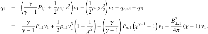$\begin{array}{ccc}{\mathit{q}}_{\mathrm{i}}& \mathrm{\equiv }& \left(\frac{\mathit{\gamma }}{\mathit{\gamma }\mathrm{-}\mathrm{1}}{\mathit{P}}_{\mathrm{i}\mathit{,}\mathrm{1}}\mathrm{+}\frac{\mathrm{1}}{\mathrm{2}}{\mathit{\rho }}_{\mathrm{i}\mathit{,}\mathrm{1}}{\mathit{v}}_{\mathrm{1}}^{\mathrm{2}}\right){\mathit{v}}_{\mathrm{1}}\mathrm{-}\left(\frac{\mathrm{1}}{\mathrm{2}}{\mathit{\rho }}_{\mathrm{i}\mathit{,}\mathrm{2}}{\mathit{v}}_{\mathrm{2}}^{\mathrm{2}}\right){\mathit{v}}_{\mathrm{2}}\mathrm{-}{\mathit{q}}_{\mathrm{e}\mathit{,}\mathrm{ad}}\mathrm{-}{\mathit{q}}_{\mathrm{B}}\\ & \mathrm{=}& \end{array}$(A.1)On the other hand it seems unphysical to assume that heat flows from one component of the plasma to another if there is no difference in heat between the two components. We can make this explicit by specifying that the heat flow between ions and electrons must be proportional to the difference between q_i and the equivalent quantity for the electrons, q_e. This difference is given by $\begin{array}{ccc}\mathrm{\Delta }\mathit{q}\mathrm{=}{\mathit{q}}_{\mathrm{i}}\mathrm{-}{\mathit{q}}_{\mathrm{e}}& \mathrm{=}& \left(\frac{\mathit{\gamma }}{\mathit{\gamma }\mathrm{-}\mathrm{1}}\right){\mathit{P}}_{\mathrm{i}\mathit{,}\mathrm{1}}{\mathit{v}}_{\mathrm{1}}\mathrm{+}\frac{\mathrm{1}}{\mathrm{2}}{\mathit{\rho }}_{\mathrm{i}\mathit{,}\mathrm{1}}{\mathit{v}}_{\mathrm{1}}^{\mathrm{3}}\left(\mathrm{1}\mathrm{-}\frac{\mathrm{1}}{{\mathit{\chi }}^{\mathrm{2}}}\right)\mathrm{-}{\mathit{q}}_{\mathrm{e}\mathit{,}\mathrm{ad}}\mathrm{-}{\mathit{q}}_{\mathrm{B}}\mathrm{-}\left[\left(\frac{\mathit{\gamma }}{\mathit{\gamma }\mathrm{-}\mathrm{1}}\right){\mathit{P}}_{\mathrm{e}\mathit{,}\mathrm{1}}{\mathit{v}}_{\mathrm{1}}\mathrm{+}\frac{\mathrm{1}}{\mathrm{2}}{\mathit{\rho }}_{\mathrm{e}\mathit{,}\mathrm{1}}{\mathit{v}}_{\mathrm{1}}^{\mathrm{3}}\left(\mathrm{1}\mathrm{-}\frac{\mathrm{1}}{{\mathit{\chi }}^{\mathrm{2}}}\right)\mathrm{+}{\mathit{q}}_{\mathrm{e}\mathit{,}\mathrm{ad}}\right]\\ & \mathrm{=}& \left(\frac{\mathit{\gamma }}{\mathit{\gamma }\mathrm{-}\mathrm{1}}\right)\mathrm{[}{\mathit{n}}_{\mathrm{i}\mathit{,}\mathrm{1}}\mathit{k}{\mathit{T}}_{\mathrm{i}\mathit{,}\mathrm{1}}\mathrm{-}{\mathit{n}}_{\mathrm{e}\mathit{,}\mathrm{1}}\mathit{k}{\mathit{T}}_{\mathrm{e}\mathit{,}\mathrm{1}}{\mathrm{(}\mathrm{2}{\mathit{\chi }}^{\mathit{\gamma }\mathrm{-}\mathrm{1}}\mathrm{-}{\mathrm{1}}^{\mathrm{)}}}^{\mathrm{]}}{\mathit{v}}_{\mathrm{1}}\mathrm{+}\frac{\mathrm{1}}{\mathrm{2}}{\mathit{m}}_{\mathrm{p}}\left({\mathit{n}}_{\mathrm{i}\mathit{,}\mathrm{1}}{\mathit{\mu }}_{\mathrm{i}}\mathrm{-}{\mathit{n}}_{\mathrm{e}\mathit{,}\mathrm{1}}{\mathit{\mu }}_{\mathrm{e}}\right){\mathit{v}}_{\mathrm{1}}^{\mathrm{3}}\left(\mathrm{1}\mathrm{-}\frac{\mathrm{1}}{{\mathit{\chi }}^{\mathrm{2}}}\right)\mathrm{-}{\mathit{v}}_{\mathrm{1}}\frac{{\mathit{B}}_{\mathrm{\perp }\mathit{,}\mathrm{1}}^{\mathrm{2}}}{\mathrm{4}\mathit{\pi }}\left(\mathit{\chi }\mathrm{-}\mathrm{1}\right)\mathit{.}\end{array}$(A.2)We can now quantify the heat flux exchange between electrons and ions in terms of this difference by adding ξΔq to Eq. (9), ξ being the fraction of the enthalpy-flux difference between ions and electrons that is used to heat the electrons: $\begin{array}{ccc}\left(\frac{\mathit{\gamma }}{\mathit{\gamma }\mathrm{-}\mathrm{1}}{\mathit{P}}_{\mathrm{e}\mathit{,}\mathrm{2}}\mathrm{+}\frac{\mathrm{1}}{\mathrm{2}}{\mathit{\rho }}_{\mathrm{e}\mathit{,}\mathrm{2}}{\mathit{v}}_{\mathrm{2}}^{\mathrm{2}}\right){\mathit{v}}_{\mathrm{2}}\mathrm{=}\left(\frac{\mathit{\gamma }}{\mathit{\gamma }\mathrm{-}\mathrm{1}}{\mathit{P}}_{\mathrm{e}\mathit{,}\mathrm{1}}\mathrm{+}\frac{\mathrm{1}}{\mathrm{2}}{\mathit{\rho }}_{\mathrm{e}\mathit{,}\mathrm{1}}{\mathit{v}}_{\mathrm{1}}^{\mathrm{2}}\right){\mathit{v}}_{\mathrm{1}}\mathrm{+}{\mathit{q}}_{\mathrm{e}\mathit{,}\mathrm{ad}}\mathrm{+}\mathit{\xi }\mathrm{\Delta }\mathit{q,}& & \end{array}$(A.3)and subtracting the same term from the ion-enthalpy flux: $\begin{array}{ccc}\left(\frac{\mathit{\gamma }}{\mathit{\gamma }\mathrm{-}\mathrm{1}}{\mathit{P}}_{\mathrm{i}\mathit{,}\mathrm{2}}\mathrm{+}\frac{\mathrm{1}}{\mathrm{2}}{\mathit{\rho }}_{\mathrm{2}}{\mathit{v}}_{\mathrm{2}}^{\mathrm{2}}\right){\mathit{v}}_{\mathrm{2}}\mathrm{=}\left(\frac{\mathit{\gamma }}{\mathit{\gamma }\mathrm{-}\mathrm{1}}{\mathit{P}}_{\mathrm{i}\mathit{,}\mathrm{1}}\mathrm{+}\frac{\mathrm{1}}{\mathrm{2}}{\mathit{\rho }}_{\mathrm{i}\mathit{,}\mathrm{1}}{\mathit{v}}_{\mathrm{1}}^{\mathrm{2}}\right){\mathit{v}}_{\mathrm{1}}\mathrm{-}{\mathit{q}}_{\mathrm{B}}\mathrm{-}{\mathit{q}}_{\mathrm{e}\mathit{,}\mathrm{ad}}\mathrm{-}\mathit{\xi }\mathrm{\Delta }\mathit{q}\mathit{.}& & \end{array}$(A.4)Assuming that the upstream electron and ion temperatures are equal we obtain the following expressions for the downstream electron and ion temperatures: $\begin{array}{ccc}\frac{\mathit{k}{\mathit{T}}_{\mathrm{e}\mathit{,}\mathrm{2}}}{{\mathit{\mu }}_{\mathrm{e}}{\mathit{m}}_{\mathrm{p}}{\mathit{v}}_{\mathrm{1}}^{\mathrm{2}}}& \mathrm{=}& \frac{\mathrm{1}}{\mathit{\gamma }{\mathit{M}}_{\mathrm{s}}^{\mathrm{2}}}\left(\frac{\mathit{\mu }}{{\mathit{\mu }}_{\mathrm{e}}}\right)\left\{{\mathit{\chi }}^{\mathit{\gamma }\mathrm{-}\mathrm{1}}\mathrm{+}\mathit{\xi }\left[\left(\frac{{\mathit{n}}_{\mathrm{i}\mathit{,}\mathrm{1}}}{{\mathit{n}}_{\mathrm{e}\mathit{,}\mathrm{1}}}\right)\mathrm{-}\mathrm{(}\mathrm{2}{\mathit{\chi }}^{\mathit{\gamma }\mathrm{-}\mathrm{1}}\mathrm{-}{\mathrm{1}}^{\mathrm{)}}\right]\right\}\mathrm{+}\frac{\mathrm{1}}{\mathrm{2}}\left(\frac{\mathit{\gamma }\mathrm{-}\mathrm{1}}{\mathit{\gamma }}\right)\left(\mathrm{1}\mathrm{-}\frac{\mathrm{1}}{{\mathit{\chi }}^{\mathrm{2}}}\right)\left\{\mathrm{1}\mathrm{+}\mathit{\xi }\left[\left(\frac{{\mathit{n}}_{\mathrm{i}\mathit{,}\mathrm{1}}}{{\mathit{n}}_{\mathrm{e}\mathit{,}\mathrm{1}}}\right)\left(\frac{{\mathit{\mu }}_{\mathrm{i}}}{{\mathit{\mu }}_{\mathrm{e}}}\right)\mathrm{-}\mathrm{1}\right]\right\}\\ & & \mathrm{-}\mathit{\xi }\frac{\mathrm{2}}{\mathit{\beta \gamma }{\mathit{M}}_{\mathrm{s}}^{\mathrm{2}}}\left(\mathrm{1}\mathrm{+}\frac{{\mathit{n}}_{\mathrm{i}\mathit{,}\mathrm{1}}}{{\mathit{n}}_{\mathrm{e}\mathit{,}\mathrm{1}}}\frac{{\mathit{\mu }}_{\mathrm{i}}}{{\mathit{\mu }}_{\mathrm{e}}}\right)\left(\frac{\mathit{\gamma }\mathrm{-}\mathrm{1}}{\mathit{\gamma }}\right)\left(\mathit{\chi }\mathrm{-}\mathrm{1}\right)\mathit{,}\\ \frac{\mathit{k}{\mathit{T}}_{\mathrm{i}\mathit{,}\mathrm{2}}}{{\mathit{\mu }}_{\mathrm{i}}{\mathit{m}}_{\mathrm{p}}{\mathit{v}}_{\mathrm{1}}^{\mathrm{2}}}& \mathrm{=}& \frac{\mathrm{1}}{\mathit{\gamma }{\mathit{M}}_{\mathrm{s}}^{\mathrm{2}}}\left(\frac{\mathit{\mu }}{{\mathit{\mu }}_{\mathrm{i}}}\right)\left\{\mathrm{1}\mathrm{-}\left(\frac{{\mathit{n}}_{\mathrm{e}\mathit{,}\mathrm{1}}}{{\mathit{n}}_{\mathrm{i}\mathit{,}\mathrm{1}}}\right)\mathrm{(}{\mathit{\chi }}^{\mathit{\gamma }\mathrm{-}\mathrm{1}}\mathrm{-}{\mathrm{1}}^{\mathrm{)}}\mathrm{-}\mathit{\xi }\left[\mathrm{1}\mathrm{-}\left(\mathrm{1}\mathrm{+}\frac{{\mathit{n}}_{\mathrm{e}\mathit{,}\mathrm{1}}}{{\mathit{n}}_{\mathrm{i}\mathit{,}\mathrm{1}}}\frac{{\mathit{\mu }}_{\mathrm{e}}}{{\mathit{\mu }}_{\mathrm{i}}}\right)\mathrm{(}\mathrm{2}{\mathit{\chi }}^{\mathit{\gamma }\mathrm{-}\mathrm{1}}\mathrm{-}{\mathrm{1}}^{\mathrm{)}}\right]\right\}\mathrm{+}\frac{\mathrm{1}}{\mathrm{2}}\left(\mathrm{1}\mathrm{-}\frac{\mathrm{1}}{{\mathit{\chi }}^{\mathrm{2}}}\right)\left(\frac{\mathit{\gamma }\mathrm{-}\mathrm{1}}{\mathit{\gamma }}\right)\left\{\mathrm{1}\mathrm{-}\mathit{\xi }\left[\mathrm{1}\mathrm{-}\left(\frac{{\mathit{n}}_{\mathrm{e}\mathit{,}\mathrm{1}}}{{\mathit{n}}_{\mathrm{i}\mathit{,}\mathrm{1}}}\right)\left(\frac{{\mathit{\mu }}_{\mathrm{e}}}{{\mathit{\mu }}_{\mathrm{i}}}\right)\right]\right\}\\ & & \mathrm{-}\left(\mathrm{1}\mathrm{-}\mathit{\xi }\right)\frac{\mathrm{2}}{\mathit{\beta \gamma }{\mathit{M}}_{\mathrm{s}}^{\mathrm{2}}}\left(\mathrm{1}\mathrm{+}\frac{{\mathit{n}}_{\mathrm{e}\mathit{,}\mathrm{1}}}{{\mathit{n}}_{\mathrm{i}\mathit{,}\mathrm{1}}}\frac{{\mathit{\mu }}_{\mathrm{e}}}{{\mathit{\mu }}_{\mathrm{i}}}\right)\left(\frac{\mathit{\gamma }\mathrm{-}\mathrm{1}}{\mathit{\gamma }}\right)\left(\mathit{\chi }\mathrm{-}\mathrm{1}\right)\mathrm{·}\end{array}$Combining these two equations gives the electron-ion temperature ratio $\begin{array}{ccc}\frac{{\mathit{T}}_{\mathrm{e}\mathit{,}\mathrm{2}}}{{\mathit{T}}_{\mathrm{i}\mathit{,}\mathrm{2}}}\mathrm{=}\left(\frac{{\mathit{\mu }}_{\mathrm{e}}}{{\mathit{\mu }}_{\mathrm{i}}}\right)\frac{\left(\frac{\mathit{\mu }}{{\mathit{\mu }}_{\mathrm{e}}}\right){\mathit{\chi }}^{\mathrm{2}}\left\{{\mathit{\chi }}^{\mathit{\gamma }\mathrm{-}\mathrm{1}}\mathrm{+}\mathit{\xi }\left[\left(\frac{{\mathit{n}}_{\mathrm{i}\mathit{,}\mathrm{1}}}{{\mathit{n}}_{\mathrm{e}\mathit{,}\mathrm{1}}}\right)\mathrm{-}\mathrm{(}\mathrm{2}{\mathit{\chi }}^{\mathit{\gamma }\mathrm{-}\mathrm{1}}\mathrm{-}{\mathrm{1}}^{\mathrm{)}}\right]\right\}\mathrm{+}{\mathit{M}}_{\mathrm{s}}^{\mathrm{2}}\left(\mathit{\gamma }\mathrm{-}\mathrm{1}\right)\mathrm{(}{\mathit{\chi }}^{\mathrm{2}}\mathrm{-}\mathrm{1}\mathrm{)}\left\{\mathrm{1}\mathrm{+}\mathit{\xi }\left[\left(\frac{{\mathit{n}}_{\mathrm{i}\mathit{,}\mathrm{1}}}{{\mathit{n}}_{\mathrm{e}\mathit{,}\mathrm{1}}}\right)\left(\frac{{\mathit{\mu }}_{\mathrm{i}}}{{\mathit{\mu }}_{\mathrm{e}}}\right)\mathrm{-}\mathrm{1}\right]\right\}\mathrm{-}\mathit{\xi }\frac{\mathrm{4}}{\mathit{\beta \gamma }}\left(\mathrm{1}\mathrm{+}\frac{{\mathit{n}}_{\mathrm{i}\mathit{,}\mathrm{1}}}{{\mathit{n}}_{\mathrm{e}\mathit{,}\mathrm{1}}}\frac{{\mathit{\mu }}_{\mathrm{i}}}{{\mathit{\mu }}_{\mathrm{e}}}\right)\left(\mathit{\gamma }\mathrm{-}\mathrm{1}\right){\mathit{\chi }}^{\mathrm{2}}\left(\mathit{\chi }\mathrm{-}\mathrm{1}\right)}{\left(\frac{\mathit{\mu }}{{\mathit{\mu }}_{\mathrm{i}}}\right){\mathit{\chi }}^{\mathrm{2}}\left\{\mathrm{1}\mathrm{-}\left(\frac{{\mathit{n}}_{\mathrm{e}\mathit{,}\mathrm{1}}}{{\mathit{n}}_{\mathrm{i}\mathit{,}\mathrm{1}}}\right)\left({\mathit{\chi }}^{\mathit{\gamma }\mathrm{-}\mathrm{1}}\mathrm{-}\mathrm{1}\right)\mathrm{-}\mathit{\xi }\left[\mathrm{1}\mathrm{-}\left(\frac{{\mathit{n}}_{\mathrm{e}\mathit{,}\mathrm{1}}}{{\mathit{n}}_{\mathrm{i}\mathit{,}\mathrm{1}}}\right)\left(\mathrm{2}{\mathit{\chi }}^{\mathit{\gamma }\mathrm{-}\mathrm{1}}\mathrm{-}\mathrm{1}\right)\right]\right\}\mathrm{-}\left(\mathrm{1}\mathrm{-}\mathit{\xi }\right)\frac{\mathrm{4}}{\mathit{\beta \gamma }}\left(\mathrm{1}\mathrm{+}\frac{{\mathit{n}}_{\mathrm{e}\mathit{,}\mathrm{1}}}{{\mathit{n}}_{\mathrm{i}\mathit{,}\mathrm{1}}}\frac{{\mathit{\mu }}_{\mathrm{e}}}{{\mathit{\mu }}_{\mathrm{i}}}\right)\left(\mathit{\gamma }\mathrm{-}\mathrm{1}\right){\mathit{\chi }}^{\mathrm{2}}\left(\mathit{\chi }\mathrm{-}\mathrm{1}\right)}\mathrm{·}& & \\ & & \end{array}$(A.7)It can be easily verified that setting ξ = 0 results in Eq. (31).

All Figures

Fig. 1 Electron-ion temperature ratio expected for minimum electron-heating (solid black line, Eq. (13)), for the case of adiabatic heating of the electrons (dashed black line, Eq. (22)), and for magnetised plasmas with β = 0.01,0.1,1 (blue dashed line, Eq 31). In addition the expected ratio is shown if on top of various thermodynamic effects there is energy exchange between the electrons and ions at the level of 5% (magenta dashed line, Eq. (A.7)). For the calculation here it is assumed that the plasma consists of electrons, protons, and fully ionised helium, and the ion temperature is the average temperature of abundance weighted temperature of the protons and helium ions. The data points are from the compilation by Ghavamian et al. (2013), and represent measured values of the electron-ion temperature ratio behind the Earth bowshock (green circles, original data from Schwartz et al. 1988), Saturn’s bowshock as measured by the Cassini spacecraft (X-shaped symbols, Masters et al. 2013) and supernova remnants (red, solid squares, van Adelsberg et al. 2008). Note that for the supernova remnants the Mach numbers are not measured, but instead the estimated shock velocity has been divided by assumed interstellar sound speed of 11 km s-1 (Ghavamian et al. 2013).

In the text

Fig. 2 Ratio of the electron temperature upstream and downstream (Te,2/Ti,2), resulting from different assumptions. The dashed line corresponds to Eq. (19) (adiabatic heating and thermalisation), the solid line corresponds to Eq. (10). For illustrative purposes we also show the effect of adiabatic compression alone (dotted line) and the upstream and upstream temperature ratios for ions (dot-dashed line).

In the text

Fig. 3 Electron-ion temperature ratio as a function of cosmic ray acceleration efficiency. The efficiency is defined here as the fraction w2 of post-shock cosmic-ray pressure (assumed here to be characterised by an adiabatic index of γcr = 1.5) to the overall pressure. The cosmic-ray efficiency is linked to the Mach number at the sub-shock, which has been affected by the compression of the plasma in the cosmic-ray precursor. See Vink et al. (2010) and Vink & Yamazaki (2014) for details.

In the text

References

- Bale, S. D., Mozer, F. S., & Horbury, T. S. 2003, Phys. Rev. Lett., 91, 265004 [NASA ADS] [CrossRef] [Google Scholar]
- Balogh, A., & Treumann, R. A. 2013, Physics of Collisionless Shocks, 1st edn. (Heidelberg, Berlin, New York: Springer-Verlag) [Google Scholar]
- Blasi, P., Morlino, G., Bandiera, R., Amato, E., & Caprioli, D. 2012, ApJ, 755, 121 [NASA ADS] [CrossRef] [Google Scholar]
- Broersen, S., Vink, J., Miceli, M., et al. 2013, A&A, 552, A9 [NASA ADS] [CrossRef] [EDP Sciences] [Google Scholar]
- Bykov, A. M., & Uvarov, Y. A. 1999, J. Exp. Theor. Phys., 88, 465 [NASA ADS] [CrossRef] [PubMed] [Google Scholar]
- Bykov, A. M., Paerels, F. B. S., & Petrosian, V. 2008, Space Sci. Rev., 134, 141 [NASA ADS] [CrossRef] [Google Scholar]
- Cargill, P. J., & Papadopoulos, K. 1988, ApJ, 329, L29 [NASA ADS] [CrossRef] [Google Scholar]
- Furuzawa, A., Ueno, D., Hayato, A., et al. 2009, ApJ, 693, L61 [NASA ADS] [CrossRef] [Google Scholar]
- Ghavamian, P., Laming, J. M., & Rakowski, C. E. 2007, ApJ, 654, L69 [NASA ADS] [CrossRef] [Google Scholar]
- Ghavamian, P., Schwartz, S. J., Mitchell, J., Masters, A., & Laming, J. M. 2013, Space Sci. Rev., 178, 633 [NASA ADS] [CrossRef] [Google Scholar]
- Helder, E. A., Vink, J., & Bassa, C. G. 2011, ApJ, 737, 85 [NASA ADS] [CrossRef] [Google Scholar]
- Itoh, H. 1978, PASJ, 30, 489 [NASA ADS] [Google Scholar]
- Laming, J. M., Hwang, U., Ghavamian, P., & Rakowski, C. 2014, ApJ, 790, 11 [CrossRef] [Google Scholar]
- Markevitch, M. 2006, in The X-ray Universe 2005, ESA SP, 604, 723 [Google Scholar]
- Masters, A., Stawarz, L., Fujimoto, M., et al. 2013, Nat. Phys., 9, 164 [NASA ADS] [CrossRef] [Google Scholar]
- Rakowski, C. E., Ghavamian, P., & Hughes, J. P. 2003, ApJ, 590, 846 [NASA ADS] [CrossRef] [Google Scholar]
- Rakowski, C. E., Laming, J. M., & Ghavamian, P. 2008, ApJ, 684, 348 [NASA ADS] [CrossRef] [Google Scholar]
- Raymond, J. C., Blair, W. P., & Long, K. S. 1995, ApJ, 454, L31 [NASA ADS] [CrossRef] [Google Scholar]
- Raymond, J. C., Vink, J., Helder, E. A., & de Laat, A. 2011, ApJ, 731, L14 [NASA ADS] [CrossRef] [Google Scholar]
- Russell, H. R., McNamara, B. R., Sanders, J. S., et al. 2012, MNRAS, 423, 236 [NASA ADS] [CrossRef] [Google Scholar]
- Schwartz, S. J., Thomsen, M. F., Bame, S. J., & Stansberry, J. 1988, J. Geophys. Res., 93, 12923 [NASA ADS] [CrossRef] [Google Scholar]
- Sollerman, J., Ghavamian, P., Lundqvist, P., & Smith, R. C. 2003, A&A, 407, 249 [NASA ADS] [CrossRef] [EDP Sciences] [Google Scholar]
- Spitzer, L. 1965, Physics of Fully Ionized Gases, 2nd edn. (New York: Interscience) [Google Scholar]
- Tidman, D. A., & Krall, N. A. 1971, Shock waves in collisionless plasmas (New York: Wiley) [Google Scholar]
- van Adelsberg, M., Heng, K., McCray, R., & Raymond, J. C. 2008, ApJ, 689, 1089 [CrossRef] [Google Scholar]
- Vink, J. 2012, A&ARv, 20, 49 [Google Scholar]
- Vink, J., & Yamazaki, R. 2014, ApJ, 780, 125 [NASA ADS] [CrossRef] [Google Scholar]
- Vink, J., Laming, J. M., Gu, M. F., Rasmussen, A., & Kaastra, J. 2003, ApJ, 587, 31 [Google Scholar]
- Vink, J., Yamazaki, R., Helder, E. A., & Schure, K. M. 2010, ApJ, 722, 1727 [NASA ADS] [CrossRef] [Google Scholar]
- Zel’dovich, Y., & Raizer, Y. P. 1966, Elements of Gasdynamics and the Classical Theory of Shock Waves (New York: Academic Press), eds. W. D. Hayes, & R.F. Probstein [Google Scholar]