| Issue |
A&A
Volume 577, May 2015
|
|
|---|---|---|
| Article Number | A36 | |
| Number of page(s) | 25 | |
| Section | Extragalactic astronomy | |
| DOI | https://doi.org/10.1051/0004-6361/201425527 | |
| Published online | 28 April 2015 | |
A sample of weak blazars at milli-arcsecond resolution⋆
1
Max-Planck-Institut für Radioastronomie,
Auf dem Hügel 69,
53121
Bonn,
Germany
e-mail:
This email address is being protected from spambots. You need JavaScript enabled to view it.
2
Istituto di Radioastronomia – INAF, via Gobetti 101,
40129
Bologna,
Italy
3
Observatorio Astronòmico, Universitat de València,
Parc Científic, C. Catedrático José Beltrán 2,
46980 Paterna, València, Spain
4
Departament d’Astronomia i Astrofísica, Universitat de
València, C. Dr. Moliner 50, 46100
Burjassot, València, Spain
Received: 16 December 2014
Accepted: 14 February 2015
Abstract
Aims. We started a follow-up investigation of the “Deep X-ray Radio Blazar Survey” objects with declination >-10 deg to better understand the blazar phenomenon. We undertook a survey with the European Very Long Baseline Interferometry Network at 5 GHz to make the first images of a complete sample of weak blazars, aiming at a follow-up comparison between high- and low-power samples of blazars.
Methods. We observed 87 sources with the EVN at 5 GHz during the period October 2009 to May 2013. The observations were correlated at the Max-Planck-Institut für Radioastronomie and at the Joint Institute for VLBI in Europe. The correlator output was analysed using both the
 and DIFMAP software packages.
Results. All of the sources observed were detected. Point-like sources are found in 39 cases on a milli-arcsecond scale, and 48 show core-jet structure. The total flux density distribution at 5 GHz has a median value ⟨ S ⟩ = 44+23-10 mJy. A total flux density ≤150 mJy is observed in 68 out of 87 sources. Their brightness temperature Tb ranges between 107 K and 1012 K. According to the spectral indices previously obtained with multi-frequency observations, 58 sources show a flat spectral index, and 29 sources show a steep spectrum or a spectrum peaking at a frequency around 1−2 GHz. Adding to the DXRBS objects we observed those already observed with ATCA in the Southern sky, we found that 14 blazars and a Steep Spectrum Radio Quasars, are associated to γ-ray emitters.
Conclusions. We found that 56 sources can be considered blazars. We also detected 2 flat spectrum narrow line radio galaxies. About 50% of the blazars associated to a γ-ray object are BL Lacs, confirming that they are more likely detected among blazars γ-emitters. We confirm the correlation found between the source core flux density and the γ-ray photon fluxes down to fainter flux densities. We also found that weak blazars are also weaker γ-ray emitters compared to bright blazars. Twenty-two sources are SSRQs or Compact Steep-spectrum Sources, and 7 are GigaHz Peaked Sources. The available X-ray ROSAT observations allow us to suggest that CSS and GPS quasars are not obscured by large column of cold gas surrounding the nuclei. We did not find any significant difference in X-ray luminosity between CSS and GPS quasars.
Key words: galaxies: active / quasars: general / BL Lacertae objects: general
Appendix A is available in electronic form at http://www.aanda.org
© ESO, 2015
1. Introduction
Less than 10% of all the active galactic nuclei (AGN) is composed of flat spectrum radio quasars (FSRQs) and BL Lacertae (BL Lac) objects. Together, these two classes of objects are named blazars. Their broad band emission, mainly generated by synchrotron and inverse-Compton radiation, extends from radio to γ rays. Blazars are characterised by high luminosity, rapid variability, and high polarisation. The majority of blazars are core-dominated objects that show apparent superluminal speeds. They are also well known γ-ray sources. The Fermi Gamma-ray Space Telescope (GST) has detected 1064 objects located at | b | > 10 deg associated to blazars based on data accumulated over the first two years of the mission: second Fermi-LAT (2FGL) catalogue (Nolan et al. 2012). The hint that relativistic Doppler boosting is connected to γ-ray detection in AGN was suggested by many authors: e.g. Kellermann et al. (2004), Kovalev et al. (2005), Taylor et al. (2007), Lister et al. (2011), and Ackermann et al. (2011).
Bright blazars are the target of many programmes for both single-dish and interferometric observations in the radio band. One of the largest samples of bright AGNs is the MOJAVE programme. It regularly observes with the Very Long Baseline Array sources with flux density >1.5 Jy (see Lister et al. 2011 and references therein).
Several of the available small size blazar samples grounded for statistical studies were selected at flux densities ~1 Jy in the radio band and a few times 10-13 erg cm-2 s-1 in X-ray band.
EVN observing sessions.
To increase the knowledge on blazars, a deeper, sizable sample has been assembled by Perlman et al. (1998) and by Landt et al. (2001), the “Deep X-ray Radio Blazar Survey” (DXRBS), which is later discussed in Padovani et al. (2007). The DXRBS sample is currently the faintest and largest blazar sample with nearly complete optical identifications including both flat spectrum radio quasars (FSRQs) and BL Lac sources. The objects were selected cross-correlating all serendipitous X-ray sources in the ROSAT database WGACAT95 (White et al. 1995) with several radio catalogues, namely GB6 (Gregory et al. 1996), North20CM (White & Becker 1992), and the 6 cm Parks-MIT-NRAO catalogue PMN (Griffith & Wright 1993), plus a snapshot survey with the Australian Telescope Compact Array (ATCA). The adopted selection criteria were a) X-ray flux in the range ~10-14−~10-12 erg cm-2 s-1 depending on the region of the sky surveyed by ROSAT; b) a two-point spectral index α ≤ 0.7; c) flux densities >100 mJy at 20 cm and >50 mJy at 6 cm.
For a deeper understanding of the blazar phenomenon, we started a follow-up investigation of the DXRBS objects, aiming at a comparison between high- and low-power samples of blazars. We first made simultaneous flux density measurements with the Effelsberg 100-m telescope at 2.64 GHz, 4.85 GHz, 8.35 GHz, and/or 10.45 GHz of all DXRBS sources with declination >−20 deg to properly compute their spectral index. Those measurements also allowed us to check for flux density variability comparing them with previous measurements found in the literature (Mantovani et al. 2011).
Since it is reasonable to expect that the objects in the DXRBS are potential γ-ray sources detected by the Fermi-GST, information on their radio structure at milli-arcsecond resolution is also essential for a comparison with bright blazar samples. For that reason we then undertook a survey with the European Very Long Baseline Interferometry Network (EVN)1 at 5 GHz to obtain images of DXRBS objects, which is the subject of the present paper.
In Sect. 2 we summarise the observations and data processing. Section 3 summarises the results achieved. Discussion and conclusions are presented in Sects. 4 and 5, respectively.
2. Observations and data reduction
With the EVN we observed all the DXRBS sources with declination >− 10 deg. The list contains 87 sources selected by applying the unique criteria of a cut in declination. The pointing positions were obtained from the FIRST catalogue for 63 objects, and for the remaining sources the coordinates were from the NVSS (Mantovani et al. 2011). This sample of sources can therefore be considered as a “complete” sample that is statistically significant.
The observations made use of all the EVN telescopes available at the scheduled time. The observing setup was: frequency band 5 GHz, dual circular polarization, recording bit rate 512 Mbps, and 2-bit sampling. Each source was tracked for four to five scans, each six minutes long at different hour angles for a better coverage of the u,v plane. About 30 min of observing time per source allow images to be produced down to an rms noise of ~0.02 mJy/beam for good network performance. Information on the observing sessions from EM077a to EM097b are reported in Table 1.
2.1. Data reduction
The EVN observations were correlated at the DiFX software correlator (Deller et al. 2011) of the Max-Planck-Institut für Radioastronomie (Bonn, Germany), and those in real time (e-EVN)2 were correlated at the Joint Institute for VLBI in Europe (Dwingeloo, The Netherlands). The raw data, output from the correlator, were integrated for one second, corresponding to a field of view of about 11′′. Table 1 shows that the sample of sources was observed with patchy telescope arrays. Moreover, we had telescopes that were affected by bad weather during the observing sessions or by abnormal functioning of the data acquisition terminals. Data provided in those cases were not particularly good so were often discarded. As a result, the rms noise values in the images are rather disperse, as reported in Table 3.
The correlator output was calibrated in amplitude and phase using 3 and imaged using DIFMAP4 (Shepherd et al. 1995). Total power measurements taken at the same times as the observations and the gain curve of the telescopes were applied in the amplitude calibration process. The visibilities of each individual data set were displayed baseline-by-baseline and carefully edited, which gave a reading of bad data. To check for other problems that affect the data, closure phases, which are defined as the sum of visibility phases around a close triangle of three antennas, were also inspected. In all cases, the source showed up at the centre of the plotted field when generating the first dirty map. The self-calibration procedure, which uses closure amplitude to determine telescope amplitude corrections, was applied. The images were produced using the difference mapping technique, in which the observer converge on a model by progressively cleaning the residual map, and self-calibrating the phases using the latest model. The model was subtracted from the data in the u-v plane at any iteration, thus avoiding aliasing of the side lobe within the field of view. The cleaning was done on a small window around the brightest component found in the residual map.
2.2. Comments on individual observing sessions
The self-calibration procedure, which uses closure amplitudes to determine telescope amplitude corrections, gave calibration for EM077a factors within 20% of unity for all the telescopes except Sh, Ur, and Wb. The often insufficient coverage of the u,v plane in particular for the longest baselines to Sh and Ur, may explain this behaviour. The reasons for the poor calibration of data provided by Wb are unclear.
EM077b and EM077c were rather unsuccessful. Several telescopes did not provide useful data. Consequently, the images obtained from these observations were not considered. The sources in both the observing lists were re-observed at a later stage, with the exception of J1332.7+4722 and J1213.0+3248, for which images were made using these data sets.
In EM077d four telescopes did not provide fringes. The calibration factors were within 20% of unity for the remaining successful telescopes.
In EM077e all telescopes worked properly and the calibration factors for the amplitude corrections were within 20% with the exception of Cm, Mc, and Jb, which required larger factors. The correction factors found were consistent for both fringe finders observed during that session.
In EM077f all stations provided data. However, their quality was often lower than expected. The closure amplitudes method showed that large calibration factors were required for most of the stations.
EM097a was quite successful. All stations provided good data. The amplitude corrections were within 20% for all telescopes but Jb and Hh.
Finally, EM097b was less successful. In particular the data acquired for the unique fringe finder, namely 4C 454.3, were rather poor. As a result, not only was the calibration in amplitude not satisfactory, but also many amplitude and phase solutions failed in fringe-fitting the data.
3. Results
3.1. Milli-arcsecond structures and spectral indices
All of the 87 sources observed have been detected. Among them, point-like sources are found in 39 cases, and 48 show core-jet structure. Examples are presented in Fig. 1. The classification of the sources based on their milli-arcsecond (mas) structure and on the spectral indices5 previously reported by Mantovani et al. (2011) is shown in Table 2 where the spectral indices have been defined as “Ultra Steep” in case of α> 0.7, “Steep” when α = 0.7−0.5, “Steep-flat” when α is steep at lower frequencies and flat tens at higher frequencies, “Flat-steep” when α is flat at lower frequencies and steep at higher frequencies, “Flat” when α< 0.5, Giga-Hertz Peaked (GPS) when the shape is convex with a peak at about the intermediate observing frequencies, and “Inverted” when the spectral index shape is mainly straight and the flux density clearly increases with frequency. The 56 objects with flat or inverted spectral index (α< 0.5) can be considered bona fide blazars. Two are flat-spectrum narrow line radio galaxies (NLRGs). Sources that show ultra-steep and steep spectral index (α> 0.5), are most probably steep spectrum radio quasars (SSRQs) or compact steep spectrum sources (CSSs).
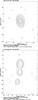 |
Fig. 1 Total-intensity images of the point-like source J0427.2−0756, the core-jet source J0126.2−0500. The convolution beams are 7.6 × 4.3 mas at 14.8 deg, 6 × 6 mas, respectively. |
Source structure and spectral index.
Derived parameters.
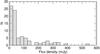 |
Fig. 2 Histogram of the frequency distribution of the flux density measurements by the EVN at 5 GHz. Two points at 742.5 mJy and 2378.0 mJy are off the plot. |
3.2. Derived parameters
Source parameters derived from the present EVN observations are reported in Table 3 for each source. The total flux density distribution has a mean value of 120 ± 273 mJy and a median value  mJy. Sixty-eight out of 87 sources show a total flux density ≤150 mJy (see Fig. 2). In Table 3 we also report the core flux density and the core size as derived using the task JMFIT. The ratio between the EVN flux density at 5 GHz from the present observations to the Effelsberg flux density previously measured by Mantovani et al. (2011) shows a median value ⟨ R ⟩ = 0.36 ± 0.08, suggesting the presence of more extended structures around the compact detected objects. The vast majority of sources shows R< 1, while only 11 sources have R> 1. The Effelsberg and the EVN flux density measurements were taken in different periods. Therefore, flux density variability and uncertainties in the EVN flux density measurements should be taken into account.
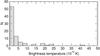 |
Fig. 3 Histogram of the frequency distribution of the brightness temperature Tb. Two points at 82.5 × 10¹⁰ K and 110.00 × 10¹⁰ K are off the plot. |
3.3. Brightness temperature
The measurements of both flux density and size of the core at mas scale, together with the available red shift (Perlman et al. 1998; Landt et al. 2001) allowed us to calculate lower limits of the brightness temperature Tb. Tb ranges between 107 K and 1012 K. The mean value is 6 ± 16 × 1010 K and the median ⟨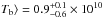 K. There are 19 sources that are unresolved when deconvolved by the beam. The mean and median values of their Tb are 7 ± 7 × 10¹⁰ K and ⟨
 K, respectively. In Fig. 3), all the values of Tb are plotted together. The large majority show a value of Tb quite low, while 13 sources show Tb> 1011 K. These values might increase when observing sources at higher resolution. Only one object, J0937.1+5008, associated to a γ-ray object detected by Fermi (see below) has Tb close to 1012 K. This source also exhibits variability by a factor of about 2.3 in flux density at 5 GHz when comparing the Effelsberg flux density to the EVN flux density, which were taken a few months apart.
4. Discussion
It is widely accepted that the γ-ray emission is produced close to the origin of the jet in highly beamed relativistic jets associated with AGN (Dermer & Schlickeiser 1994; Fuhrmann et al. 2014). High angular-resolution images are therefore critical for our understanding of the mechanism that generates such high-energy radiation, therefore a systematic comparison of the γ-ray and radio properties for a complete sample of blazars is mandatory. Models have been suggested that predict that the γ-ray sources have more highly relativistic jets and are aligned close to the line of sight (e.g. Lister & Marscher 1997; Jorstad et al. 2001; Kellermann et al. 2004). Evidence that the observed γ-ray flares are associated with the ejection of new superluminal components in AGN and that a γ-ray event occurs within the jet features was reported by Jorstad et al. (2001). To this aim, the parsec-scale jet kinematic properties of AGN, and the correlation of the γ-ray flux with quasi-simultaneous parsec-scale radio flux density in the MOJAVE sample associated with bright γ-ray sources detected by the Fermi-GST, have been discussed by Lister et al. (2009) and Kovalev et al. (2009). As a consequence, about 100 sources selected amongst those detected by the Large Area Telescope on-board the Fermi-GST with S15 GHz> 100 mJy were added to the list of sources in the VLBA MOJAVE programme monitoring.
We made the first parsec-scale resolution observations of a complete sample of blazars selected from the faintest DXRBS by applying the only criteria of a cut in declination at >−10 deg. The sample is formed by 87 objects, ~13% of which are BL Lacs. All sources were detected, confirming they actually are compact objects. Mantovani et al. (2011) made simultaneous multi-frequency observations to better define the radio spectral index type for the DXRBS objects. We found that 56 objects showing flat or inverted spectral index can be classified as blazars, 22 objects show steep spectral index, and 7 more objects are Giga-peaked spectral index. The 56 blazars show a median flux density  mJy. Of them 42 show a flux density S< 150 mJy at 5 GHz. They potentially represent the appropriate sample for a comparison between faint and bright blazar samples. The sample also contains two flat-spectrum NLRGs, J1120.4+5855 and J1229.5+2711.
4.1. Association to a γ-ray object
The objects in the DXRBS are distributed over the whole sky. To find any possible association between them and the 2FGL objects, we cross-checked their positions. For the 87 DXRBS objects observed in the northern sky, we improved their positional accuracy by deriving the positions from the FIRST (Becker et al. 1994) and from the NVSS (Condon et al. 1998; see Mantovani et al. 2011). For 91 DXRBS objects in the southern sky with declination <− 10 deg, the NVSS or ATCA positions are taken from Landt et al. (2001) and Perlman et al. (1998). Nine of the sources observed with the EVN show a good positional overlapping, which holds for an association between these radio sources and γ objects. Eight of the γ-ray emitters are FSRQs or BLLacs, and one is a SSRQ. Since all the DXRBS objects observed with the EVN were detected, we assume that the DXRBS sources observed with ATCA at 2 arcsec resolution are also compact objects detectable with mas interferometric observations. Six out of the 91 southern sources also show a good positional overlapping with 2FGL objects. The associations are presented in Table 5 with other useful information. All of the associations have already been suggested in the 2FGL. However, we add further characteristics for these sources suitable to possibly confirm radio-gamma identification.
Considering an association of a blazar with a γ-ray source as an identification also requires evidence of a correlation between the radio and γ light curves, the former often missing in case of weak radio sources. Three of the blazars in Table 5 are variable in both radio and γ rays. Two sources only vary in the radio band and two in the γ band. For two more objects, there is no evidence of any variability so far. Amongst sources observed with the EVN, all but one of the associated radio-gamma objects are among the 56 blazars we found, suggesting that the 14% of weak blazars are also γ-ray emitters. No information is available about variability in the radio band, while only one is reported as variable in γ-rays.
If we now take all the suggested radio-γ associations into account, about 50% of the objects listed in Table 5 are classified as BL Lac. The DXRBS contains about 13% of BL Lac objects in total, showing that BL Lacs are more likely to be detected as a γ emitter than FSRQs. As pointed out by Ackermann et al. (2011) investigating a much larger sample, this is mainly due to the different limiting flux in the γ regime for FSRQs and BL Lacs, which show soft and hard spectral indices, respectively.
Steep spectrum sources.
It is worth noting that the source J0204.8+1514 is the only SSRQ amongst those associated to a γ-ray object. This source is also classified as a possible CSS in Table 4. The angular size reported by Cooper et al. (2007) for J0204.8+1514 observed with the VLA A-array at 1.4 GHz after beam deconvolution is 1.58 arcsec as major axis, 1.42 arcsec as minor axis, at a position angle of −40.5 deg. This corresponds to a linear size LS = 4.7 kpc, which classifies it as CSS. However, Cooper et al. (2007) also find a faint extended emission above the 3σ noise level of their image. Mantovani et al. (2011) and Nolan et al. (2012) found the source variable in the radio- and γ-ray bands, respectively, which is rather peculiar in a CSS. J0204.8+1514 was included in the MOJAVE programme selected because it was classified flat spectrum source, which does not seem to be the case. VLBA observations at 15 GHz show a mas core-jet structure for J0204.8+1514.
4.2. Comparison between high- and low-power samples of blazars
An interesting by-product of this investigation is the preliminary comparison between high- and low-power samples of blazars. One of the most extended samples of bright flat spectrum blazars is the MOJAVE sample (Lister & Homan 2005; Lister et al. 2009) regularly observed with the Very Long Baseline Array6. It includes all the objects with VLBA flux density exceeding 1.5 Jy at 15 GHz, declination >− 30 deg, plus all known AGNs above declination >− 20 deg detected by Fermi and with compact flux density of at least 100 mJy at 15 GHz. An investigation of the γ-ray and 15 GHz radio properties of bright blazars reflecting a wide range of spectral energy distribution parameters was possible for blazars included in the MOJAVE programme. The synchrotron self-Compton model is favored for the γ-ray emission in BL Lac objects over external seed-photon models. FSRQs are shown to have a different behaviour.
DXRBS sources possibly associated to Fermi objects.
The association between relativistic beaming and the derived properties suggests that high-synchrotron peaked BL Lac have lower Doppler factors than lower-synchrotron peaked BL Lac objects and FSRQs (Lister et al. 2011). The present sample of weak blazars, 41 of which show Score< 100 mJy, for the time being lacks the monitoring programme needed to search for structural changes and to evaluate Doppler factors. However, the existing mas resolution observations allowed us to derive useful parameters that can be used to complement previous findings for bright blazars.
A highly significant correlation with a formal probability of a chance correlation of 5 × 10⁻⁶ was found by Pushkarev et al. (2010) between the source core flux density at 15 GHz obtained by the MOJAVE VLBA programme and the integrated 0.1−100 GeV γ-ray photon fluxes taken from the Fermi 1FGL catalogue. They analysed a large sample of 183 LAT-detected AGNs. Because the correlation is weaker if the jet flux density is used instead, they suggest that the core is the site of the γ-ray emission. Furthermore, they suggest that the region where most of γ-ray photons are produced is located within the compact opaque parsec-scale core, at a typical distance between the γ-ray production region and the 15 GHz radio core of 7 pc, in good agreement with Fuhrmann et al. (2014).
The presence of this correlation in this highly variable population further suggests that Doppler beaming is likely the cause and that Doppler factors of the individual jets are not changing substantially over time (Pushkarev et al. 2010). Because of the selection criteria followed for sources observed in the MOJAVE VLBA programme, there is a limit in the plot about 100 mJy in the core flux density. Most of the sources associated with Fermi 2FGL objects we observed with the EVN reaches a much lower level in flux densities at 5 GHz. The plot of Fig. 2 by Pushkarev et al. (2010) can be updated with these new data pairs taking two limiting factors into account: a) interferometric observations for our sample at 15 GHz are missing. However, all but one source listed in Table 5 have a flat spectral index. We can assume that their flux density at 15 GHz is similar to or even lower than the one we measured with the EVN at 5 GHz owing to the better resolution achieved with the VLBA at that frequency; b) the flux densities by Pushkarev et al. (2010) are those measured after the LAT event with a delay of about 2.5 months. Again, the information for structural changes with time for the DXRBS sources are still not available.
Keeping that in mind, we updated the Pushkarev et al. (2010) plot by adding data pairs that have the radio flux density taken from our EVN measurements and the ATCA measurements made by Perlman et al. (1998) and Landt et al. (2001) and the integrated γ-ray photon flux of the associated Fermi objects, evaluated from the fit of the full band (100 MeV−100 GeV), taken from the 2FGL catalogue (Nolan et al. 2012). The updated plot is shown in Fig. 4. Taking the uncertainties in the data pairs we added into account, the correlation is clearly confirmed. The ATCA flux densities should be considered as upper limits. Shifting those points to left in the plot should improve the correlation.
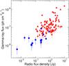 |
Fig. 4 Integrated 0.1-100GeV Fermi-LAT photon flux vs. 15 GHz VLBA core flux density as in Fig. 2 of Pushkarev et al. (2010) (triangles), complemented with data pairs from the present work (circles). |
To make sure that the method adopted for updating the plot in Fig. 4 is convincing, we also compared our data pairs with those of Fig. 1 in Linford et al. (2012), in which they plot the γ-ray photon flux versus the total VLBA radio flux density at 5 GHz for 232 sources. For the 15 associated objects of the present work, we derived the total flux densities at 5 GHz from the EVN images and from the ATCA measurements, plotting them versus the corresponding integrated γ-ray photon flux from the 2FGL catalogue. The new data pairs fit nicely into the Linford et al. (2012) plot, which also show that a strong correlation between radio flux density and γ-ray flux of blazars is in place.
Lister (2010) plotted the 11-month median Fermi energy flux against VLBA 15 GHz flux density for the first Fermi-MOJAVE sample (1FM). The bottom left-hand quadrant of Fig. 1 of that paper shows that more than half of the γ-ray-limited 1FM sample consists of AGN that are not in the flux-limited MOJAVE sample, implying that they have lower-than-average radio-to-γ-ray flux ratio. All of them lie below the MOJAVE limit of 1.5 Jy. Lister suggests that a possible explanation is that the weaker γ-ray emission from blazars is boosted by a higher Doppler factor than their radio emission, as for the proposed external Compton model by Dermer (1995). Adding the data pairs from the present work to Lister’s plot, they fill the bottom left-hand quadrant, a clear indication that weak blazars are also weak γ-ray emitters. Therefore invoking the external Compton model to explain the lack of faint γ-ray emitters may not be needed. The Fermi observations (1FGL 2008-08-04–2009-07-04; 2FGL 2008-08-04–2010-08-01) and the EVN observations (2009-10-22–2013-05-27) can almost be considered as concurrent. However, before considering it unnecessary to apply the external Compton model, it is better to keep in mind the uncertainties incidental to data pairs from the present work.
4.3. Steep-spectrum and GigaHz-Peaked sources
Twenty-nine sources in our sample show a steep spectrum or a spectrum peaking at a frequency around 1−2 GHz (GPSs), according to Mantovani et al. (2011). We extracted their arcsecond scale sizes from the FIRST and NVSS and computed their projected linear size LS. This sub-sample of objects is listed in Table 4, together with other parameters collected from literature. Column 2 in Table 4 reports which class of objects they belong to, signally SSRQs, CSSs, GPSs, and BL Lacs.
Sources with LS ≤ 20 kpc and power P1.4 GHz> 1025 W Hz-1 are classified as CSSs or GPSs, which are young radio sources with ages <107 yr (Fanti et al. 1990). Their projected linear size LS was computed using H0 = 100 km s-1 Mpc-1 and q0 = 1, following the cosmology adopted in that paper. The source J0435.1−0811 was classified as GPS with a question mark, showing a peaked spectral index and an LS quite larger than 20 kpc.
Since X-ray ROSAT observations are available for the DXRBS objects, this sample of CSS and GPS quasars can be used for a systematic study of their X-ray properties. The X-ray luminosity is found in the range 1043−1046 erg s-1 with a median value of  erg s-1, a value that is a bit lower than the luminosity of 1045−1046 erg s-1 reported by O’Dea (1998) for CSS and GPS quasars by X-ray measurements taken by different observers. Moreover, we do not find any significant difference in X-ray luminosity between CSSs and GPS quasars. The derived column densities of hydrogen nH, resemble the Galactic nH column density, ignoring the presence of X-ray absorbing material in excess, which suggests that CSS and GPS quasars are not obscured by large column of cold gas surrounding the nuclei. The percentage of polarised emission at 8.35 or 10.45 GHz is <1% in almost all cases (see Table 4), in good agreement with the finding of Mantovani et al. (2009), who made single-dish observations with the 100-m Effelsberg telescope of a complete sample of CSSs.
Sources listed in Table 4, showing a projected LS >20 kpc are classified as SSRQs. These are objects in which the lobe emission dominates the radio core emission. Their jets are viewed at larger angles than blazars, resulting in weaker beaming effects. They show properties between those of both FSRQs and radio quiet quasars. Clearly, the faint lobe emission is resolved out by the EVN observations presented in this paper.
Table 4 also lists three objects classified as BL Lacs. This is quite unexpected since BL Lacs show flat spectral index in the radio band. It is worth mentioning that the optical classification of these three objects as BL Lacs is questionable (see Perlman et al. 1998; Landt et al. 2001)
5. Summary and conclusions
We have presented EVN observations at 5 GHz of a complete sample of 87 weak objects from the DXRBS selected with a declination >− 10 deg as the unique criterion. All of the sources were detected: 39 are point-like, 48 show a core-jet structure.
Their brightness temperature Tb ranges between 107 K and 1012 K. The large majority of them show a very low value of Tb. Thirteen sources show Tb> 1011 K. There are 19 sources that are unresolved when deconvolved by the beam. The mean and median values of their Tb are 7 ± 7 × 10¹⁰ K and  K, respectively. Only J0937.1+5008, associated to a γ-ray object, has Tb close to 1012 K.
Amongst the 87 sources observed, 56 can be considered as blazars, 22 show a steep spectral index, and 7 more objects are classified as Giga-Peaked Sources. The sample also contains two NLRGs, namely J1120.4+5855 and J1229.5+2711. The 56 blazars potentially represent an appropriate sample for a direct comparison between faint- and bright-blazar samples. They show a median flux density mJy. Of them 42 show a flux density S< 150 mJy at 5 GHz.
We found that 14 DXRBS flat spectrum objects and 1 steep spectrum object are associated to γ-ray emitters from the 2FGL. Among the radio-γ associations, about 50% of the objects are BL Lacs. The DXRBS containes about 13% of BL Lac in total. This confirms that BL Lacs are more likely to be detected among blazars γ-emitters.
The correlation found by Pushkarev et al. (2010) between the source core flux density at 15 GHz obtained by the MOJAVE VLBA programme and the 0.1−100 GeV γ-ray photon fluxes taken from the Fermi 1FGL extends to lower fluxes when adding the new data pairs of weak blazars we collected to the plot. After updating the plot by Lister (2010), data pairs from the present work fill the bottom left quadrant of the plot, indicating that weak blazars are also weaker γ-ray emitters compared to bright blazars, suggesting that they may not be needed to invoke the external Compton model. Before considering this as a firm statement, we have to keep the constraints on the added data pairs in mind.
About half of the steep or convex spectrum sources are point-like, and half show a core-jet in the FIRST or NVSS images. With linear size ≤20 kpc and power P1.4 GHz> 1025 W Hz-1, they can be classified as CSSs or GPSs, i.e. young radio sources with ages <107 yr. This sub-sample of objects with X-ray ROSAT observations can be used for a systematic study of the X-ray properties in CSS and GPS quasars. The X-ray luminosity range is 1043−1046 erg s-1 with a median value of  erg s-1, a bit lower than a luminosity of 1045−1046 erg s-1 as reported by O’Dea (1998). Any difference in X-ray luminosity between CSSs and GPS quasars is not significant. The nH column densities resemble the Galactic nH column density, suggesting that CSS and GPS quasars are not obscured by a large column of cold gas surrounding the nuclei. All of these objects are rather weakly polarised.
The DXRBS sample has the great advantage over the MOJAVE sample because it facilitates a direct comparison between γ-ray detected and non-detected sources in the same radio flux-limited sample. The present investigation can be considered as a useful basis for further monitoring programmes aiming to observe structure changes, to detect flux density variability, and to derive other parameters for weak blazars.
Online material
Appendix A: Images
In this Appendix we present the images of the 87 weak blazars observed with the EVN at 5 GHz. Map peak in mJy/beam, contours in percentage of the peak flux density in the map, and the full width half maximum (FWHM) of the beam in milli-arcseconds and the position angles of the beam major axis in degrees are reported for each image.
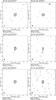 |
Fig. A.1 EVN images at 5 GHz. |
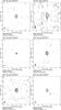 |
Fig. A.1 continued. |
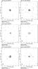 |
Fig. A.1 continued. |
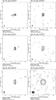 |
Fig. A.1 continued. |
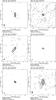 |
Fig. A.1 continued. |
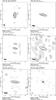 |
Fig. A.1 continued. |
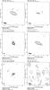 |
Fig. A.1 continued. |
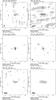 |
Fig. A.1 continued. |
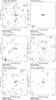 |
Fig. A.1 continued. |
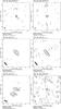 |
Fig. A.1 continued. |
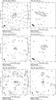 |
Fig. A.1 continued. |
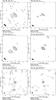 |
Fig. A.1 continued. |
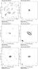 |
Fig. A.1 continued. |
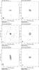 |
Fig. A.1 continued. |
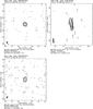 |
Fig. A.2 continued. |
The European VLBI Network is a joint facility of European, Chinese, South African and other radio astronomy institutes funded by their national research councils.
e-VLBI research infrastructure in Europe is supported by the European Union’s Seventh Framework Programme (FP7/2007-2013) under grant agreement number RI-261525 NEXPReS.
is the NRAO’s Astronomical Image Processing System.
DIFMAP is part of the Caltech VLBI software package.
The spectral index is defined as Sν ∝ ν− α.
The VLBA is a facility of the National Science Foundation operated by The National Radio Astronomy Observatory under cooperative agreement with the Associated Universities, Inc.
Acknowledgments
The research leading to these results has received funding from the European Commission Seventh Framework Programme (FP/2007-2013) under grant agreement No 283393 (RadioNet3). E.R. acknowledges partial support by the Spanish MINECO project AYA2012-38941-C02-01 and the Generalitat Valenciana project PROMETEOII/2012/057. This research has made use of data from the MOJAVE database that is maintained by the MOJAVE team (Lister et al. 2009). We are gratful to Alaksander Pushkarev for providing his data and to Lars Fuhrmann for all the suggestions while we were drafting the paper. This work made use of the Swinburne University of Technology software correlator, developed as part of the Australian Major National Research Facilities Programme and operated under licence. It has also used the NASA/IPAC Extragalactic Database (NED) which is operated by the Jet Propulsion Laboratory, California Institute of Technology, under contract with the National Aeronautics and Space Administration, and NASA’s Astrophysics Data System. We are very grateful to an anonymous referee for very helpful comments and suggestions and for a careful reading of the manuscript of this paper.
References
- Ackermann, M., Ajello, M., Allafort, A., et al. 2011, ApJ, 741, 30 [NASA ADS] [CrossRef] [Google Scholar]
- Becker, R. H., White, R. L., & Helfand, D. J. 1994, ASP Conf. Ser. 61, eds. D. R. Crabtree, R. J. Hanisch, & J. Barnes, 165 [Google Scholar]
- Condon, J. J., Cotton, W. D., Greisen, E. W., et al. 1998, AJ, 115, 1693 [NASA ADS] [CrossRef] [Google Scholar]
- Cooper, N. J., Lister, M. L., & Kochanczyk, M. D. 2007, ApJS, 171, 376 [NASA ADS] [CrossRef] [Google Scholar]
- Deller, A. T., Brisken, W. F., Phillips, C. J., et al. 2011, PASP, 123, 275 [NASA ADS] [CrossRef] [Google Scholar]
- Dermer, C. D. 1995, ApJ, 446, L63 [NASA ADS] [CrossRef] [Google Scholar]
- Dermer, C. D., & Schlickeiser, R. 1994, ApJS, 90, 945 [NASA ADS] [CrossRef] [Google Scholar]
- Fanti, R., Fanti, C., Schilizzi, R. T., et al. 1990, A&A, 231, 333 [NASA ADS] [Google Scholar]
- Fuhrmann, L., Larsson, S., Chiang, J., et al. 2014, MNRAS, 441, 1899 [NASA ADS] [CrossRef] [Google Scholar]
- Gregory, P. C., Scott, W. K., Douglas, K., & Condon, J. J. 1996, ApJS, 103, 427 [NASA ADS] [CrossRef] [Google Scholar]
- Griffith, M. R., & Wright, A. E. 1993, AJ, 105, 1666 [NASA ADS] [CrossRef] [Google Scholar]
- Jorstad, S. G., Marscher, A. P., Mattox, J. R., et al. 2001, ApJS, 134, 181 [NASA ADS] [CrossRef] [Google Scholar]
- Kellermann, K. I., Lister, M. L., Homan, D. C., et al. 2004, ApJ, 609, 539 [NASA ADS] [CrossRef] [Google Scholar]
- Kovalev, Y. Y., Kellermann, K. I., Lister, M. L., et al. 2005, AJ, 130, 2473 [NASA ADS] [CrossRef] [Google Scholar]
- Kovalev, Y. Y., Aller, H. D., Aller, M. F., et al. 2009, ApJ, 696, L17 [NASA ADS] [CrossRef] [Google Scholar]
- Landt, H., Padovani, P., Perlman, E. S., et al. 2001, MNRAS, 323, 757 [NASA ADS] [CrossRef] [Google Scholar]
- Linford, J. D., Taylor, G. B., Romani, R. W., et al. 2012, ApJ, 744, 177 [NASA ADS] [CrossRef] [Google Scholar]
- Lister, M. L. 2010, in Fermi meets Jansky – AGN in Radio and Gamma Rays, eds. T. Savolainen, E. Ros, R. W. Porcas, & J. A. Zensus (Bonn: MPIfR), 159 [Google Scholar]
- Lister, M. L., & Homan, D. C. 2005, AJ, 130, 1389 [NASA ADS] [CrossRef] [Google Scholar]
- Lister, M. L., & Marscher, A. P. 1997, ApJ, 476, 572 [NASA ADS] [CrossRef] [Google Scholar]
- Lister, M. L., Cohen, M. H., Homan, D. C., et al. 2009, AJ, 138, 1874 [NASA ADS] [CrossRef] [Google Scholar]
- Lister, M. L., Aller, M., Aller, H., et al. 2011, ApJ, 742, 27 [NASA ADS] [CrossRef] [Google Scholar]
- Mantovani, F., Mack, K.-H., Montenegro-Montes, F. M., et al. 2009, A&A, 502, 61 [NASA ADS] [CrossRef] [EDP Sciences] [Google Scholar]
- Mantovani, F., Bondi, M., & Mack, K.-H. 2011, A&A, 533, A79 [NASA ADS] [CrossRef] [EDP Sciences] [Google Scholar]
- Nolan, P. L., Abdo, A. A., Ackermann, M., et al. 2012, ApJS, 199, 31 [NASA ADS] [CrossRef] [Google Scholar]
- O’Dea, C. 1998, PASP, 110, 493 [NASA ADS] [CrossRef] [Google Scholar]
- Padovani, P., Giommi, P., Landt, H., & Perlman, E. S. 2007, ApJ, 662, 182 [NASA ADS] [CrossRef] [Google Scholar]
- Perlman, E. S., Padovani, P., Giommi, P., et al. 1998, AJ, 115, 1253 [NASA ADS] [CrossRef] [Google Scholar]
- Pushkarev, A. B., Kovalev, Y. Y., & Lister, M. L. 2010, ApJ, 722, L11 [NASA ADS] [CrossRef] [Google Scholar]
- Shepherd, M. C., Pearson, T. J., & Taylor, G. B. 1995, BAAS, 26, 305 [Google Scholar]
- Taylor, G. B., Healey, S. E., Helmboldt, J. F., et al. 2007, ApJ, 671, 1355 [NASA ADS] [CrossRef] [Google Scholar]
- White, R. L., & Becker, R. H. 1992, ApJS, 79, 331 [NASA ADS] [CrossRef] [Google Scholar]
- White, N. E., Giommi, P., & Angelini, L. 1995, http://heasarc.gsfc.nasa.gov/wgcat [Google Scholar]
All Tables
All Figures
|
Fig. 1 Total-intensity images of the point-like source J0427.2−0756, the core-jet source J0126.2−0500. The convolution beams are 7.6 × 4.3 mas at 14.8 deg, 6 × 6 mas, respectively. |
| In the text | |
|
Fig. 2 Histogram of the frequency distribution of the flux density measurements by the EVN at 5 GHz. Two points at 742.5 mJy and 2378.0 mJy are off the plot. |
| In the text | |
|
Fig. 3 Histogram of the frequency distribution of the brightness temperature Tb. Two points at 82.5 × 10¹⁰ K and 110.00 × 10¹⁰ K are off the plot. |
| In the text | |
|
Fig. 4 Integrated 0.1-100GeV Fermi-LAT photon flux vs. 15 GHz VLBA core flux density as in Fig. 2 of Pushkarev et al. (2010) (triangles), complemented with data pairs from the present work (circles). |
| In the text | |
|
Fig. A.1 EVN images at 5 GHz. |
| In the text | |
|
Fig. A.1 continued. |
| In the text | |
|
Fig. A.1 continued. |
| In the text | |
|
Fig. A.1 continued. |
| In the text | |
|
Fig. A.1 continued. |
| In the text | |
|
Fig. A.1 continued. |
| In the text | |
|
Fig. A.1 continued. |
| In the text | |
|
Fig. A.1 continued. |
| In the text | |
|
Fig. A.1 continued. |
| In the text | |
|
Fig. A.1 continued. |
| In the text | |
|
Fig. A.1 continued. |
| In the text | |
|
Fig. A.1 continued. |
| In the text | |
|
Fig. A.1 continued. |
| In the text | |
|
Fig. A.1 continued. |
| In the text | |
|
Fig. A.2 continued. |
| In the text | |
Current usage metrics show cumulative count of Article Views (full-text article views including HTML views, PDF and ePub downloads, according to the available data) and Abstracts Views on Vision4Press platform.
Data correspond to usage on the plateform after 2015. The current usage metrics is available 48-96 hours after online publication and is updated daily on week days.
Initial download of the metrics may take a while.