| Issue |
A&A
Volume 577, May 2015
|
|
|---|---|---|
| Article Number | A89 | |
| Number of page(s) | 12 | |
| Section | Interstellar and circumstellar matter | |
| DOI | https://doi.org/10.1051/0004-6361/201425228 | |
| Published online | 08 May 2015 | |
Orbital evolution of colliding star and pulsar winds in 2D and 3D: effects of dimensionality, EoS, resolution, and grid size
1
Departament d’Astronomia i MeteorologiaInstitut de Ciències del Cosmos
(ICC), Universitat de Barcelona (IEEC-UB),
Martí i Franquès 1, 08028 Barcelona
Catalonia
Spain
e-mail: This email address is being protected from spambots. You need JavaScript enabled to view it.
2
Astrophysical Big Bang Laboratory, RIKEN, 2-1 Hirosawa, Wako, 351-0198
Saitama,
Japan
e-mail: This email address is being protected from spambots. You need JavaScript enabled to view it.
3 Dept. d’Astronomia i Astrofísica, Universitat de València,
C/Dr. Moliner 50, 46100 Burjassot ( València), Spain
Received:
28
October
2014
Accepted:
23
February
2015
Abstract
Context. The structure formed by the shocked winds of a massive star and a non-accreting pulsar in a binary system suffers periodic and random variations of orbital and non-linear dynamical origins. The characterization of the evolution of the wind interaction region is necessary for understanding the rich phenomenology of these sources.
Aims. For the first time, we simulate in 3 dimensions the interaction of isotropic stellar and relativistic pulsar winds along one full orbit, on scales well beyond the binary size. We also investigate the impact of grid resolution and size, and of different state equations: a γ̂-constant ideal gas, and an ideal gas with γ̂ dependent on temperature.
Methods. We used the code PLUTO to carry out relativistic hydrodynamical simulations in 2 and 3 dimensions of the interaction between a slow dense wind and a mildly relativistic wind with Lorentz factor 2, along one full orbit in a region up to ~100 times the binary size. The different 2-dimensional simulations were carried out with equal and larger grid resolution and size, and one was done with a more realistic equation of state than in 3 dimensions.
Results. The simulations in 3 dimensions confirm previous results in 2 dimensions, showing: a strong shock induced by Coriolis forces that terminates the pulsar wind also in the opposite direction to the star; strong bending of the shocked-wind structure against the pulsar motion; and the generation of turbulence. The shocked flows are also subject to a faster development of instabilities in 3 dimensions, which enhances shocks, two-wind mixing, and large-scale disruption of the shocked structure. In 2 dimensions, higher resolution simulations confirm lower resolution results, simulations with larger grid sizes strengthen the case for the loss of the general coherence of the shocked structure, and simulations with two different equations of state yield very similar results. In addition to the Kelvin-Helmholtz instability, discussed in the past, we find that the Richtmyer-Meshkov and the Rayleigh-Taylor instabilities are very likely acting together in the shocked flow evolution.
Conclusions. Simulations in 3 dimensions confirm that the interaction of stellar and pulsar winds yields structures that evolve non-linearly and become strongly entangled. The evolution is accompanied by strong kinetic energy dissipation, rapid changes in flow orientation and speed, and turbulent motion. The results of this work strengthen the case for the loss of the coherence of the whole shocked structure on large scales, although simulations of more realistic pulsar wind speeds are needed.
Key words: hydrodynamics / X-rays: binaries / stars: winds, outflows / radiation mechanisms: non-thermal / gamma rays: stars
© ESO, 2015
1. Introduction
As already proposed long ago, binary systems hosting a massive star and a powerful non-accreting pulsar can produce gamma rays through the interaction of the stellar and the pulsar winds (e.g. Maraschi & Treves 1981). An actual instance of this kind of object is the binary system PSR B1259−63(/LS2883), which consists of a late O star with a decretion disc (Negueruela et al. 2011) and a 47 ms pulsar (Johnston et al. 1992), and which is a powerful GeV and TeV emitter (e.g. Aharonian et al. 2005; Abdo et al. 2011; Tam et al. 2011). Other binaries emitting gamma rays may also pertain to this class, such as LS 5039, LS I +61 303, HESS J0632+057, and 1FGL J1018.6−5856 (see e.g. Barkov & Khangulyan 2012; Paredes et al. 2013; Dubus 2013, and references therein), although the true nature of the compact object in these sources is still unknown. In the whole Galaxy, if taking a lifetime for the non-accreting pulsar of a few times 105 yr (the age of PSR B1259−63) and the birth rates for high-mass binaries hosting a neutron star (e.g. Portegies Zwart & Yungelson 1999), one might expect ~100 of these systems (see also Paredes et al. 2013; Dubus 2013).
The rich phenomenology of PSR B1259−63/LS288 (see Chernyakova et al. 2014, for a multi-wavelength study of the 2010 periastron passage), and (possibly) also of other gamma-ray binaries, is directly linked to the complex processes taking place in the colliding wind region. To study this complexity, several works have already been devoted to the numerical study of the wind collision region, neglecting or including orbital motion, and on scales similar or beyond those of the binary (Romero et al. 2007; Bogovalov et al. 2008, 2012; Okazaki et al. 2011; Takata et al. 2012; Bosch-Ramon et al. 2012; Bogovalov et al. 2012; Lamberts et al. 2012b,a, 2013; Paredes-Fortuny et al. 2015). In particular, in Bosch-Ramon et al. (2012) the authors performed two-dimensional (2D) simulations in planar coordinates of the interaction of a dense, non-relativistic stellar wind and a powerful, mildly relativistic pulsar wind along one full orbit, up to scales ≈ 40 times the orbital separation distance (here orbit semi-major axis a). These simulations showed the early stages of the spiral structure also found in non-relativistic simulations (Lamberts et al. 2012b), but the fast growth of instabilities (see also Lamberts et al. 2013) and strong two-wind mixing have suggested the eventual disruption of the spiral and the isotropization of the mass, momentum, and energy fluxes (as predicted in Bosch-Ramon & Barkov 2011).
If the results from Bosch-Ramon et al. (2012) were confirmed, it would imply several important facts: the two-wind interaction is subject to strongly non-linear processes already within the binary system; the isotropization of the interaction region leads to loss of coherence on scales not far beyond a, eventually becoming a more or less irregular isotropic flow formed by mixed stellar and pulsar winds; this mixed flow terminates with a shock on the external medium (interstellar medium (ISM) or the interior of a supernova remnant (SNR); see Bosch-Ramon & Barkov 2011). All these dynamical processes would imply the existence of many potential sites for particle acceleration, such as shocks, turbulence, shear flows, and non-thermal emission, mainly synchrotron and inverse Compton, from deep inside the system on pc scales.
In this work, we go a step forward in the study of the interaction of the stellar and the pulsar winds with orbital motion. We have performed the first three-dimensional (3D), relativistic simulations using similar parameters to those adopted in Bosch-Ramon et al. (2012) up to a distance ~30 a from the binary. The results obtained in 3D are compared with results found in new 2D simulations in planar coordinates under the same conditions, in particular the same grid size and number of cells in each direction. Additional 2D simulations were also carried out to study the effects of a more realistic equation of state (EoS), higher resolution, and a larger grid size up to ~100 a from the binary, not reached so far in relativistic simulations.
2. Numerical simulations
2.1. Simulation code: PLUTO
The simulations were implemented in 3D and 2D with the PLUTO code1 (Mignone et al. 2007), the piece-parabolic method (PPM; Colella & Woodward 1984), and an HLLC Riemann solver (Mignone & Bodo 2005). PLUTO is a modular Godunov-type code entirely written in C and intended mainly for astrophysical applications and high Mach number flows in multiple spatial dimensions. For this work, it was run through the MPI library in the CFCA cluster of the National Astronomical Observatory of Japan.
2.2. Gas equation of state
The simulated flows were approximated in most of the cases as an ideal, relativistic adiabatic gas with no magnetic field, one particle species, and a constant polytropic index of 4/3 (CtGa), since using such a simple EoS reduces the time cost of the simulations carried out. One 2D simulation (model 2Dlf; see Table 1) was also carried out with an adaptive Synge-type EoS (Taub 1978) for a one particle species, non-degenerate, relativistic gas (Mignone et al. 2005), to check the impact of a more complex EoS on the shocked two-wind structure. A generalized, more complete treatment of the EoS leads to changes in the Rankine-Hugoniot conditions and gas thermodynamical properties, in particular for the stellar wind. Because the latter is dense and cold enough, thermal cooling could also be important (see Sect. 4). This more complete treatment of the gas is left for future work.
2.3. Resolution and grid size
We adopted a changing resolution in the 3D simulations (model 3Dlf; see Table 1) to reach larger scales. The computational domain size is x ∈ [−32 a,32 a], y ∈ [−32 a,32 a], and z ∈ [−10 a,10 a]. The 3D domain has a resolution of 512 × 512 × 256 cells. The central part of this domain, x ∈ [−2 a,2 a], y ∈ [−2 a,2 a], and z ∈ [−a,a], has a resolution of 256 × 256 × 128 cells, and outside this domain the cell size grows exponentially2 with distance outwards in each direction. The equivalent uniform resolution for the whole domain would be 4096 × 4096 × 2560 cells. The adopted resolution came from a compromise between computational costs and a maximum Lorentz factor. The 3D simulations required about 3 × 10⁵ cpu h on NAOJ cluster XC30. To achieve higher Lorentz factors, say ≈ 10, we should have doubled the grid resolution (see Sect. 3.1 in Bosch-Ramon et al. 2012), in particular in the central region, leading to a much longer computation (see Sect. 4). Adaptive mesh refinement (AMR) was not implemented for these simulations, because in the considered problem, the AMR technique fills most of the computational volume with the smallest scale grid owing to the growth of turbulence. Nested-grid AMR could avoid such behaviour, but abrupt changes in resolution can produce unphysical pressure jumps. Nevertheless, the chosen geometry in our calculations, with an exponential growth of the grid cells outwards, naturally follows the spatial scales of the hydrodynamical processes, which smoothly grow outwards with respect to the system.
Parameters of the models considered in this work.
2.4. Additional simulation models
We performed four additional 2D simulations to compare the influence of equation of state, geometry dimensionality, grid resolution, and size. Model 2Dlf has the same domain size and resolution distribution as 3Dlf in the X and Y directions. Model 2Dle has the same domain size and resolution distribution as 2Dlf in the X and Y directions, but makes use of Taub. Model 2Dhf has the same domain size but twice the resolution of 2Dlf. Finally, model 2Dhbf has an increased computational domain of x ∈ [−100 a,100 a] and y ∈ [−100 a,100 a] (as before, central regions are x ∈ [−2 a,2 a] and y ∈ [−2 a,2 a]), and a better effective resolution with a cell distribution: Nx = [512,512,512] and Ny = [512,512,512] cells (equivalent uniform resolution: 25 600 × 25 600), where the first number shows the resolution in the region with negative coordinates, the second one is the resolution in the uniform central region, and the third one is the resolution in the region with positive coordinates. The model details are summarized in Table 1.
2.5. Simulated physics
The pulsar-to-star wind momentum rate ratio, η = Ṗpw/Ṗsw, was fixed to 0.1 in 3D. This value for η is a standard value for the case of a massive star and a powerful pulsar (e.g. Bosch-Ramon & Barkov 2011; Bosch-Ramon et al. 2012; Dubus 2013). For a meaningful geometric comparison between the 3D and 2D results on scales ~a, we set  to locate the two-wind contact discontinuity (CD) at the same distance from the pulsar (Rp), as
  where d is the separation distance between the two stars. Under negligible pressure, the momentum rates are
  for the pulsar and the stellar winds, respectively; Γ, ρpw and β are the pulsar wind Lorentz factor, rest-frame density, and c-normalized velocity; and ρsw and vsw the stellar wind density and velocity. The pulsar spin-down luminosity can be approximated as
  Both winds are injected with spherical symmetry, and their pressure at injection can be considered negligible. In particular for the case of the pulsar wind, the pressure was chosen as low as allowed by the numerical scheme.
A Γ-value of two was adopted. Our value of the Lorentz factor is the same as the one taken by Bosch-Ramon et al. (2012), and it yields high wind-density and velocity contrasts in the two-wind contact discontinuity (CD), although still much higher than those implied by the conventional value Γ ~ 104−106 (see Khangulyan et al. 2012; Aharonian et al. 2012, and references therein). A modest Γ-value has been chosen because of resolution limitations, since the reconstruction of the fluxes can lead to negative values for the term (1−β2) if β is very close to 1. Pressure may also be affected. However, given that for Γ = 2, the amount of kinetic energy is equal to the rest-mass energy of the pulsar wind, relativistic effects start to become apparent. On the other hand, because pulsar wind Γ-values are thought to be much higher than simulated here, the development of instabilities could be different. For instance, the Kelvin-Helmholtz instability (KHI) growth is proportional to the square root of the density contrast (Chandrasekhar 1961), and Γ ~ 104−106 would imply significantly slower growth rates. The analysis of instability growth in the present scenario is numerically and physically complex, so specific thorough studies beyond the scope of this work are needed, but it is worth noting that 2D simulations with Γ = 10 gave qualitatively similar results to those with Γ = 2 (see Sect. 3.1, and Bosch-Ramon et al. 2012). A detailed discussion of the impact of relativistic effects on the shocked-wind structure can be found in Bosch-Ramon et al. (2012). In the same paper, there is also a discussion of the KHI development with different flow velocities (see also Lamberts et al. 2013). In addition to the KHI, we also note below the development of the Richtmyer-Meshkov (e.g. Richtmyer 1960; Meshkov 1969; Brouillette 2002; Nishihara et al. 2010; Inoue 2012; Matsumoto & Masada 2013) and the Rayleigh-Taylor instabilities (e.g. Taylor 1950; Chandrasekhar 1961), acting together (RMI+RTI) at the orbit-leading side of the two-wind CD. The RMI+RTI, not considered before, are less dependent on the density contrast than the KHI and should not be strongly affected even if Γ were much larger than adopted. It is worth noting that for the shocked relativistic pulsar wind, it is inertia rather than density what matters, but the stellar wind still dominates the growth of the RMI+RTI, and so it occurs in the non-relativistic regime.
Unlike Bosch-Ramon et al. (2012), who simulated a generic case, in this work the orbital elements and stellar wind velocity (vw) were taken similar to those of LS 5039 (Casares et al. 2005; Aragona et al. 2009; Sarty et al. 2011): eccentricity e = 0.24; period T = 3.9 days; orbital semi-major axis a = 2.3 × 1012 cm; and vw = 0.008 c = 2.4 × 108 cm s-1, with a stellar wind Mach number of 7 at injection. For the given η, Γ, and vw values, the stellar and pulsar wind momentum rates, normalized to the stellar mass-loss rate, Ṁ-7 = (Ṁ/10-7M⊙ yr-1), are Ṗsw ≈ 6 × 1027Ṁ-7 and Ṗpw ≈ 6 × 1026Ṁ-7 g cm s-2 (≈ 2 × 1027Ṁ-7 g cm s-2 in 2D), respectively. The corresponding spin-down luminosity in 3D is ≈ 2 × 1037Ṁ-7 erg s-1. The values of vw, Γ, Ṁ, and η determine the wind densities. Since Ṁ is not required in these adiabatic gas simulations, its value is left unconstrained, but the adopted normalization of 10-7M⊙ yr-1 is characteristic of O-type stellar winds.
The simulations do not include the magnetic field or anisotropy in the pulsar wind, although their impact should be small. In particular for the magnetic field, this should be the case at least when the magnetic-energy to particle-energy density ratio is σ ≲ 1 (see Bogovalov et al. 2012). On larger scales, the shocked mixed winds propagate in a medium with steep drops of density and pressure (Bosch-Ramon & Barkov 2011), and thus σ should remain small until the flow is terminated on pc scales. On those scales, which are much larger than those simulated here, σ may evolve as when the pulsar wind interacts directly with the ISM or the interior of a SNR, in which case magnetic lines accumulate in the nebula, making σ grow (Kennel & Coroniti 1984).
2.6. Initial setup
The simulations start running (t = 0) when the pulsar is at apastron (1.24 a,0,0) and to the right of the star (0,0,0). The orbital motion takes place in the XY-plane, and set counter-clockwise. Initially, the wind of the pulsar occupies a sphere of radius a/2, and a region bounded by a cone tangent to this sphere and oriented rightwards. The stellar wind occupies the rest of the grid. The initial setup is illustrated in Fig. 1. The injection region of the pulsar wind, which as the stellar wind is injected continuously, is taken as a sphere of radius 0.07 a. The injection region of the stellar wind has a radius of 0.15 a. Both injectors are smaller than their distances to the shocked winds at any point of the orbit. After starting the simulation, the pulsar wind injector is relocated to account for orbital motion, which is done slowly enough to avoid numerical artifacts.
The quasi-steady state of the simulation can be considered to be reached when the stellar wind shocked at t = 0 leaves the computational domain, which occurs after a simulation running time ~1/6−1/8 × T ~ 1/2 days.
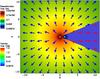 |
Fig. 1 Density distribution by colour and arrows representing the flow motion direction, in the orbital plane (XY) for 3Dlf at the beginning of the simulation (t = 0; apastron). |
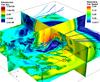 |
Fig. 2 Representation of the distribution of density in the XY-, XZ-, and YZ-planes for 3Dlf at t = 3.9 days (apastron). Streamlines are shown in 3D. |
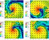 |
Fig. 3 Density distribution by colour and arrows representing the flow motion direction in the orbital plane (XY) for 3Dlf at: t = 2.6, 3.9 (apastron), 5.2, and 5.85 days (periastron) (from left to right, and top to bottom). |
3. Results
Figure 2 illustrates the 3D distribution of the density at apastron. The figure shows plane cuts in the XY-, XZ-, and YZ-planes taken after one full orbital period at t = 3.9 days. The shocked-wind structure has already reached a quasi-stationary state. Figure 3 shows the distribution of density in the orbital plane for 3Dlf at times t = 2.6, 3.9 (apastron), 5.2, and 5.85 days (periastron). For better visualizing the results of 3Dlf, a zoom in of the density distribution around the pulsar during periastron is shown in Fig. 4. Also, Fig. 5 shows the distribution of tracer (1 for the pulsar and –1 for the stellar wind, respectively), modulus of the four-velocity spatial component (γβ), and Mach number, for 3Dlf in the same plane. For completeness, Fig. 6 presents the density distribution for plane cuts along the star-pulsar axis and perpendicular to the orbital plane at the same times as those in Fig. 3. In addition, Fig. 7 provides the density distribution at periastron for plane cuts perpendicular to the orbital plane at different angles from the star-pulsar axis and clockwise: φ = 0,π/4,π/2, 3π/4.
Figure 8 shows the distribution of density on the orbital plane for the same times as those in Fig. 3 for model 2Dlf. The same is shown in Fig. 9, but for a simulation with increased resolution and grid size (2Dhbf), and with slightly different orbital phases. Figure 10 shows the distribution of tracer, γβ, and Mach number, for 2Dhbf. Figure 11 allows for the comparison when using two different EoS: CtGa and Taub. Finally, Fig. 12 allows the comparison of the density distribution at the same orbital phase (t = 5.85 days) for the models 3Dlf, 2Dlf, 2Dhf, and 2Dhbf (see Table 1).
3.1. 3D case
The quasi-stationary solution of the 3D simulation confirms what has already been seen in 2D using planar coordinates in Bosch-Ramon et al. (2012). Despite some quantitative differences discussed below, Figs. 2−5 display the same features as those found by Bosch-Ramon et al. (2012).
3.1.1. Coriolis forces and instabilities
On one hand, instabilities starting at ~2 a from the pulsar quickly develop in the CD. These instabilities may have two different origins. Owing to the velocity difference between the two shocked winds, their origin may be the KHI. Also, because the two media have very different densities and are subject to recurrent lateral shaking and persistent acceleration provided by the Coriolis force, the instability may be driven mostly by RMI+RTI. All these instabilities could couple together, and also with the orbital motion-induced Coriolis force, which pushes material from the CD to stop the propagation of the shocked pulsar wind coming from within the binary. This is apparent, for instance, at the leading edge of the shocked-wind structure at the point where the CD widens due to the instabilities (see Fig. 4).
The importance of RMI+RTI is also suggested by the presence of turbulence in the leading edge of the shocked flow structure, and by its almost complete absence in the traling edge. The process can be explained as follows. As the pulsar orbits the star, the underdense shocked pulsar wind penetrates the much denser shocked stellar wind, causing the RTI to develop. Because the pulsar wind shock rotates in the direction of the CD, it can catch up with the RTI fingers and trigger the development of the RMI. Unlike the KHI, the RMI+RTI are less dependent on the density contrast and could have a similar strength even for much higher Γ-values.
After termination within the binary, the shocked pulsar wind reaccelerates to become supersonic, and then a strong shock forms again when its path is blocked by the disrupted CD, heavily loaded with shocked stellar wind. The mass load of the pulsar wind region is very apparent in the figures as abrupt and patchy changes in density and tracer starting at ~5−10 a from the pulsar. This material from the CD penetrates further, stopping the unshocked pulsar wind moving away from the star with an almost perpendicular shock.
Despite the relevant role of the hydrodynamical instabilities, we note that the Coriolis force is the main factor that shapes the interaction region, inducing the strong asymmetry of the shocked-wind structure, as seen in Fig. 4. It is the very effect of the Coriolis force that makes the shocked flow propagation outwards strongly non-ballistic, creating quasi-perpendicular shocks at the termination of the pulsar wind behind the pulsar (as seen from the star). Once shocked, the flow deviates strongly, following the trend imposed by the material against which it shocked, starting the spiral pattern (counter-orbitwise). These shocks do not have the same nature as the oblique shocks terminating the pulsar wind behind the pulsar found in axisymmetric, non-relativistic and relativistic simulations of the same scenario but without orbital motion (e.g., Bogovalov et al. 2008; Lamberts et al. 2011). In particular, in axisymmetric cases the termination shock behind the pulsar disappears for η ≳ 0.012, whereas here η = 0.1. The Coriolis shocks found in our simulations are also different from those generated behind the pulsar when this is moving in the ISM (e.g. Bucciantini et al. 2005), since the environment in that case has a constant density. To finish with, as noted below, the size of the whole shocked-wind structure clearly depends on the orbital phase, which would be difficult to explain if the KHI alone played a dominant dynamical role. Because the RMI+RTI are fueled by the Coriolis force, these instabilities are actually actively participating in shaping the asymmetric shape of the whole two-wind interaction region.
3.1.2. Evolution on larger scales
The orbital motion leads to a spiral-like structure, as expected. However, the coherence of this structure is strongly affected by the unstable nature of the flow, which is rich in strong shocks and mixing induced by the Coriolis force, as predicted in Bosch-Ramon & Barkov (2011) and suggested by the numerical results of Bosch-Ramon et al. (2012). We must note, however, that low resolution on the larger scales leads to the attenuation of shocks and turbulence and to the enhancement of mixing.
The present 3D results strengthen the thesis that the spiral shape is eventually lost, because the structure almost gets disrupted already within the grid, on scales ~30 a. This is supported by Figs. 2−7, in which the lowest density regions of the arm of the spiral seem to split into different branches.
The complexity of the matter distribution is best illustrated in the plane cuts perpendicular to the orbital plane in Figs. 2, 6, and 7, which also show how the pulsar wind is terminated at moderately different distances from the pulsar depending on latitude. This is explained by the different pressure found by the pulsar wind, depending on the angle with which it faces the Coriolis force. The opening angle of the shocked-wind structure is determined by the Coriolis force on the orbital plane, whereas in the perpendicular direction, the opening angle is ~60°, as in the case without orbital motion (e.g. Bogovalov et al. 2008). However, the KHI and RMI+RTI starting in the CD lead to fluctuations in the opening angle in this direction and, on larger scales, the shocked-wind structure becomes wider, since the high sound speed of the shocked gas allows the latter to quickly transfer thrust to the vertical direction.
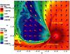 |
Fig. 4 Zoom in of the region around the pulsar region at periastron shown in Fig. 3. Two labels pointing to the two edges, leading and trailing, of the shocked structure are shown. |
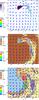 |
Fig. 5 Distribution of tracer, γβ, and Mach number (from top to bottom) for 3Dlf at t = 5.2 days. |
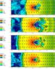 |
Fig. 6 Density distribution by colour, and arrows representing the flow motion direction in the plane perpendicular to the orbit and crossing the star-pulsar axis, for 3Dlf at: t = 2.6, 3.9 (apastron), 5.2, and 5.85 days (periastron; from top to bottom). |
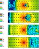 |
Fig. 7 Density distribution by colour and arrows representing the flow motion direction in a plane perpendicular to the orbit for 3Dlf at t = 5.85 days (periastron). The panels show different slices with an angle φ from the star-pulsar axis and clockwise: φ = 0,π/4,π/2, 3π/4 (from top to bottom). |
We point out that in the vertical cuts what could be mostly distorting the CD should be KHI rather than RMI+RTI, as one would expect that the impact of the Coriolis force should diminish with latitude. As seen in the perpendicular cuts of Figs. 6 and 7, variations in d and in the pulsar angular velocity along the moderately eccentric orbit yield almost proportional variations in Rp and in the size of the whole interaction region. In particular, the ratio of d between apastron and periastron passages is ≈ 1.8, whereas the whole interaction region size changes by a factor ≈ 1.6 in our simulations. Therefore, although size changes induced by instabilities are also taking place, as shown in Figs. 6 and 7 and also in Fig. 3, the region size evolves correlated with the orbital motion.
3.2. Comparison of 2D and 3D results
The results shown in Figs. 8 and 9 are very similar to those obtained by Bosch-Ramon et al. (2012) from 2D simulations with slightly different orbital parameters, and are also qualitatively very much like the 3D results just presented. As noted, the main features of the quasi-stationary solution in 2D and 3D are the same. The density distribution maps of Figs. 3 and 8 and in the top panel of Fig. 12 allow for a comparison of results in 2D and 3D at periastron with the same resolution: the wind from the pulsar terminates closer to the pulsar in the opposite direction to the star, but it is wider in 3D than in 2D. Shocks, mixing, and turbulence start earlier, and mixing and turbulence seem to be much stronger in 3D. All this is also seen when comparing Figs. 5 and 10.
The different η-values adopted in 3D and 2D, 0.1 versus 0.11/2 (see Sect. 2), imply higher mass, momentum and energy fluxes for the pulsar wind in 2D, so it can explain why in 3D the termination of the pulsar wind and triggering of flow disruptive phenomena are closer to the pulsar. The higher strength of the disruptive phenomena in 3D would be, on the other hand, motivated by the higher number of geometric degrees of freedom. The wider opening angle of the unshocked pulsar wind region in 3D (see Fig. 12) could be explained by the stronger dilution of the shocked pulsar wind in the trailing edge of the interaction region.
3.3. Effects of higher resolution
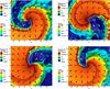 |
Fig. 8 Density distribution by colour, and arrows representing the flow motion direction, for 2Dlf at: t = 2.6, 3.9 (apastron), 5.2, and 5.85 days (periastron; from left to right, and top to bottom). |
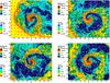 |
Fig. 9 Density distribution by colour, and arrows representing the flow motion direction, for 2Dhbf at: t = 4.8, 6.3, 7.0, and 9.85 days (~periastron; from left to right, and top to bottom). |
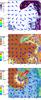 |
Fig. 10 Distribution of tracer, γβ, and Mach number (from top to bottom) for 2Dhbf at t = 5.2 days. |
Figures 12, 8, and 9 (top right and bottom left and right panels) allow for a comparison of the impact of increasing the resolution on the simulation results. Qualitatively, the higher resolution does not change the shocked-wind structure significantly and, as when comparing 3D and 2D simulations, the same major features are present in all the simulations: (i) fast RMI+RTI and possibly KHI growth at the CD; (ii) strong shocks terminating both the unshocked and the shocked pulsar wind; (iii) bending of the whole structure; (iv) development of turbulence; (v) and strong two-wind mixing. However, with an increase in resolution, the instability growth is quicker, which leads to more turbulence downstream in the spiral and also to pulsar wind termination closer to the pulsar as turbulent material from the CD exerts more pressure from one side (see Perucho et al. 2004, for a general study of the resolution influence on the evolution of KHI in numerical calculations). Given the higher dimensionality, a quicker instability development in 3D is expected, terminating the pulsar wind in the opposite direction to the star and generating turbulence even closer to the pulsar, if the resolution is increased. This must nevertheless be tested in future work with an even higher resolution and a more realistic pulsar-wind Lorentz factor.
3.4. Effects of a larger grid
Figure 9 shows the density distribution evolution for the 2D simulation with the largest grid and the highest effective resolution. The maps show how the spiral starts disrupting through the growth of the KHI, RMI, and RTI, which favours two-wind mixing and structure deformation. In addition, different spiral arms are connected through channels of lower density, while the spiral arms themselves seem to lose their integrity. This 2D simulation strongly suggests that in 3D, the structure would lose coherence even closer (< 100 a) to the binary. The effects on these scales with a mildly relativistic pulsar wind in 2D are similar to those obtained by Lamberts et al. (2012b) also in 2D for the non-relativistic case and specific regions of the parameter space, but the Newtonian nature of those simulations makes a comparison difficult.
3.5. Effects of a different EoS
Figure 11 allows for the comparison in 2D of using two different EoS, a single-species, ideal relativistic gas with constant  , and an adaptive Synge-type EoS for a one particle-species, non-degenerate, relativistic gas. Despite the different gas physics of the interacting flows, the figure shows that the results are almost identical in both cases, with only moderate changes in size for the inner region of the shocked-wind structure, in particular regarding the thickness of the shocked wind regions, which are thicker in the Taub case. Accordingly, the densities of the shocked flows also reach moderately lower values in the Taub case. All this is expected because the compression ratio is smaller for a non- (
 ) or a mildly (
 ) relativistic wind than in the ultrarelativistic case, when : from 4 to 7. This is also the reason for the Coriolis shock occurring slightly closer to the pulsar in the Taub case, since the shocked pulsar wind region is slightly thicker in that case.
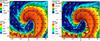 |
Fig. 11 Comparison of the density distribution at t = 3.1 days between 2Dlf (left), and 2Dle (right), corresponding respectively to an ideal relativistic gas with constant |
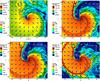 |
Fig. 12 Comparison of the density distribution (colour), and flow motion direction (arrows), in the orbital plane (XY) at t = 5.85 days (periastron) for 3Dlf, 2Dlf, 2Dhf, and 2Dhbf (from left to right, and top to bottom). |
4. Discussion and summary
The results presented here suggest that the shocked-wind structure is already very unstable on scales ~10 a. In addition to structure bending, flow reacceleration, and full pulsar wind termination (all features found in both 2D and 3D simulations), the instabilities affecting the CD, possibly KHI and RMI+RTI, grow faster in 3D. This leads to turbulence and to shocks further downstream in the outflowing shocked winds, and also to efficient matter mixing that leads to more shocks, because dense clumps of stellar material penetrate into the region occupied by the fast and light shocked pulsar wind.
Many of the results of this work have already been found in previous 2D simulations (Bosch-Ramon et al. 2012), but in 3D all the processes occur closer to the binary. An enhancement of the resolution should make the interaction region more unsteady, likely shortening further the distances on which the RMI+RTI and KHI develop, and enhancing two-wind mixing even more. It is interesting to note that the bending length in 3D is about three times longer than the point of balance between the Coriolis force and the pulsar wind ram pressure (see Eq. (9) in Bosch-Ramon & Barkov 2011). This is expected because the perturbations triggered by reaching pressure balance at the leading edge of the CD need time to transfer energy and momentum to the whole shocked-wind structure.
On larger scales, ~10−100 a, the radial pressure gradient suffered by the shocked two-wind flow triggers strong RTI with the instabilitiy fingers growing radially. This is already hinted at in 3Dlf but is more clear seen in 2Dhbf, to the extent that arms of the spiral formed by the orbital motion disrupt and mix. This environment, which is still relatively close to the star to have enough radiation targets but also large enough to be resolvable in radio, is very rich in candidate sites for non-thermal emission (see the discussion in Bosch-Ramon et al. 2012; see also the semi-analytical study at high energies of Zabalza et al. 2013) for which Doppler boosting can be an issue given the non-uniform velocity distribution. In particular, as seen for instance in Figs. 3 and 9, shocked pulsar wind material is found to move straight along quite large distances (~10 a). Since this material is shocked, it has a likely content of non-thermal particles. Owing to the proximity to the star, these particles could quickly radiate their energy through inverse Compton scattering. This radiation, given the at least mildly relativistic velocities, could be Doppler boosted by a factor of ~16γ2 ≳ 10 for an observer viewing the flow with an angle < 1 /γ from its axis, where γ is the Lorentz factor. For large systems such as PSR B1259–63, X-rays could also be useful for observationally probing the shocked-wind structure on scales of ~1017 cm (Kargaltsev et al. 2014). For smaller systems and/or on larger scales (Durant et al. 2011), one may study the bubble in the surrounding medium fed by the shocked two-wind flow (Bosch-Ramon & Barkov 2011).
It is noteworthy that, owing to momentum and energy isotropization, the evolution of the shocked-wind structure in the perpendicular direction gets broader further downstream than in the case without orbital motion. The study of this process deserves specific simulations with a larger grid in the Z direction. In the same line, a more accurate characterization of the evolution of the shocked-wind structure (velocities, shocks, turbulence, mixing and general coherence) along the orbit would deserve higher resolution and eventually a larger grid size, despite being computationally very costly.
Our 3D simulations are capturing some relevant features of the shocked-wind structure but the increase of the grid resolution is a natural future step. For instance, to increase the Lorentz factor of the pulsar wind by a factor of a few, the resolution of the central part of the computational domain should be doubled. In addition, as hinted at by the 2D simulations (see Fig. 12), the large scale turbulence would be well resolved with three to four times more resolution in the grid than in our current 3D setup. This can be justified by a minimum cell size close to the typical gyroradius of the shocked pulsar wind particles: ~3 × 10⁹ETeV/BG cm, where ETeV is the particle energy in TeV and BG the magnetic field in G. This applies if one assumes that the physical dissipation scales are near the particle gyroradius, which is reasonable for a shocked pulsar wind consisting of an ideal collisionless plasma with low B and with realistic Γ-values. However, such an increase in resolution would require about 107 cpu hours. This is a demanding calculation, but we plan to carry it out as it is a necessary step in the characterization of the scenario under study3.
Among other less costly improvements there would be to use a more realistic EoS, although our preliminary study shows only minor differences between using CtGA and Taub. Thermal cooling should also be included since the shock of the stellar wind may be radiative, making the collision region more unstable and favouring mixing of the CD and its disruption (Pittard 2009). This is likely to increase turbulence and the presence of shocks in the shocked pulsar wind region even further. More feasible, but requiring the simplification of the region containing the system, is the simulation of the interaction of the shocked-wind structure with the environment on large scales, which was predicted to take place as a fast dense non-relativistic wind colliding with the surrounding medium (Bosch-Ramon & Barkov 2011).
Finally, another important line of research is computing the emission from the shocked flows using the hydrodynamical information, which could be carried out first in the test-particle approximation. Another improvement would be to carry relativistic simulations with an anisotropic and/or inhomogeneous stellar wind4, such as adding an equatorial disc, because several of the known gamma-ray binaries host Be stars. Finally, VLBI radio data are very important for observationally characterizing the shocked-wind structure on the simulated scales (e.g. Moldón et al. 2011b,a, 2012).
We mean here average improvement, although in the grid periphery, the resolution would still be significantly below the ideal case.
Regarding anisotropic and/or inhomogeneous (clumpy) stellar winds, see Paredes-Fortuny et al. (2015) for the axisymmetric case, and Okazaki et al. (2011), Takata et al. (2012) for the non-relativistic case.
Acknowledgments
The calculations were carried out in the CFCA cluster of National Astronomical Observatory of Japan. We thank Andrea Mignone and the PLUTO team for the possibility to use the PLUTO code. We especially thank to Claudio Zanni for technical support. The visualization of the results used the VisIt package. V.B.-R. acknowledges support by the Spanish Ministerio de Economía y Competitividad (MINECO) under grants AYA2013-47447-C3-1-P. V.B.-R. also acknowledges financial support from MINECO and European Social Funds through a Ramón y Cajal fellowship. This research has been supported by the Marie Curie Career Integration Grant 321520. B.M.V. acknowledges partial support by the JSPS (Japan Society for the Promotion of Science): No. 2503786, 25610056, 26287056, 26800159. B.M.V. also acknowledges MEXT (Ministry of Education, Culture, Sports, Science and Technology): No. 26105521 and RFBR grant 12-02-01336-a. M.P. is a member of the working team of projects AYA2013-40979-P and AYA2013-48226-C3-2-P, funded by the Spanish Ministerio de Economía y Competitividad.
References
- Abdo, A. A., Ackermann, M., Ajello, M., et al. 2011, ApJ, 736, L11 [NASA ADS] [CrossRef] [Google Scholar]
- Aharonian, F., Akhperjanian, A. G., Aye, K.-M., et al. 2005, A&A, 442, 1 [Google Scholar]
- Aharonian, F. A., Bogovalov, S. V., & Khangulyan, D. 2012, Nature, 482, 507 [NASA ADS] [CrossRef] [PubMed] [Google Scholar]
- Aragona, C., McSwain, M. V., Grundstrom, E. D., et al. 2009, ApJ, 698, 514 [NASA ADS] [CrossRef] [Google Scholar]
- Barkov, M. V., & Khangulyan, D. V. 2012, MNRAS, 2375 [Google Scholar]
- Bogovalov, S. V., Khangulyan, D. V., Koldoba, A. V., Ustyugova, G. V., & Aharonian, F. A. 2008, MNRAS, 387, 63 [NASA ADS] [CrossRef] [Google Scholar]
- Bogovalov, S. V., Khangulyan, D., Koldoba, A. V., Ustyugova, G. V., & Aharonian, F. A. 2012, MNRAS, 419, 3426 [NASA ADS] [CrossRef] [Google Scholar]
- Bosch-Ramon, V., & Barkov, M. V. 2011, A&A, 535, A20 [NASA ADS] [CrossRef] [EDP Sciences] [Google Scholar]
- Bosch-Ramon, V., Barkov, M. V., Khangulyan, D., & Perucho, M. 2012, A&A, 544, A59 [NASA ADS] [CrossRef] [EDP Sciences] [Google Scholar]
- Brouillette, M. 2002, Ann. Rev. Fluid Mech., 34, 445 [Google Scholar]
- Bucciantini, N., Amato, E., & Del Zanna, L. 2005, A&A, 434, 189 [NASA ADS] [CrossRef] [EDP Sciences] [Google Scholar]
- Casares, J., Ribó, M., Ribas, I., et al. 2005, MNRAS, 364, 899 [NASA ADS] [CrossRef] [Google Scholar]
- Chandrasekhar, S. 1961, Hydrodynamic and hydromagnetic stability (Oxford: Clarendon) [Google Scholar]
- Chernyakova, M., Abdo, A. A., Neronov, A., et al. 2014, MNRAS, 439, 432 [NASA ADS] [CrossRef] [Google Scholar]
- Colella, P., & Woodward, P. R. 1984, J. Comp. Phys., 54, 174 [Google Scholar]
- Dubus, G. 2013, A&ARv, 21, 64 [NASA ADS] [CrossRef] [Google Scholar]
- Durant, M., Kargaltsev, O., Pavlov, G. G., Chang, C., & Garmire, G. P. 2011, ApJ, 735, 58 [NASA ADS] [CrossRef] [Google Scholar]
- Inoue, T. 2012, ApJ, 760, 43 [NASA ADS] [CrossRef] [Google Scholar]
- Johnston, S., Manchester, R. N., Lyne, A. G., et al. 1992, ApJ, 387, L37 [Google Scholar]
- Kargaltsev, O., Pavlov, G. G., Durant, M., Volkov, I., & Hare, J. 2014, ApJ, 784, 124 [NASA ADS] [CrossRef] [Google Scholar]
- Kennel, C. F., & Coroniti, F. V. 1984, ApJ, 283, 710 [NASA ADS] [CrossRef] [Google Scholar]
- Khangulyan, D., Aharonian, F. A., Bogovalov, S. V., & Ribo, M. 2012, ApJ, 752, L17 [NASA ADS] [CrossRef] [Google Scholar]
- Lamberts, A., Fromang, S., & Dubus, G. 2011, MNRAS, 418, 2618 [NASA ADS] [CrossRef] [Google Scholar]
- Lamberts, A., Dubus, G., Fromang, S., & Lesur, G. 2012a, in AIP Conf. Ser. 1505, eds. F. A. Aharonian, W. Hofmann, & F. M. Rieger, 406 [Google Scholar]
- Lamberts, A., Dubus, G., Lesur, G., & Fromang, S. 2012b, A&A, 546, A60 [NASA ADS] [CrossRef] [EDP Sciences] [Google Scholar]
- Lamberts, A., Fromang, S., Dubus, G., & Teyssier, R. 2013, A&A, 560, A79 [NASA ADS] [CrossRef] [EDP Sciences] [Google Scholar]
- Maraschi, L., & Treves, A. 1981, MNRAS, 194, 1 [Google Scholar]
- Matsumoto, J., & Masada, Y. 2013, ApJ, 772, L1 [NASA ADS] [CrossRef] [Google Scholar]
- Meshkov, E. 1969, Fluid Dynamics, 4, 101 [NASA ADS] [CrossRef] [Google Scholar]
- Mignone, A., & Bodo, G. 2005, MNRAS, 364, 126 [NASA ADS] [CrossRef] [Google Scholar]
- Mignone, A., Plewa, T., & Bodo, G. 2005, ApJS, 160, 199 [NASA ADS] [CrossRef] [Google Scholar]
- Mignone, A., Bodo, G., Massaglia, S., et al. 2007, ApJS, 170, 228 [Google Scholar]
- Moldón, J., Johnston, S., Ribó, M., Paredes, J. M., & Deller, A. T. 2011a, ApJ, 732, L10 [NASA ADS] [CrossRef] [Google Scholar]
- Moldón, J., Ribó, M., & Paredes, J. M. 2011b, A&A, 533, L7 [NASA ADS] [CrossRef] [EDP Sciences] [Google Scholar]
- Moldón, J., Ribó, M., & Paredes, J. M. 2012, A&A, 548, A103 [NASA ADS] [CrossRef] [EDP Sciences] [Google Scholar]
- Negueruela, I., Ribó, M., Herrero, A., et al. 2011, ApJ, 732, L11 [NASA ADS] [CrossRef] [Google Scholar]
- Nishihara, K., Wouchuk, J. G., Matsuoka, C., Ishizaki, R., & Zhakhovsky, V. V. 2010, Roy. Soc. London Phil. Trans. Ser. A, 368, 1769 [NASA ADS] [CrossRef] [Google Scholar]
- Okazaki, A. T., Nagataki, S., Naito, T., et al. 2011, PASJ, 63, 893 [NASA ADS] [Google Scholar]
- Paredes, J. M., Bednarek, W., Bordas, P., et al. 2013, Astropart. Phys., 43, 301 [NASA ADS] [CrossRef] [Google Scholar]
- Paredes-Fortuny, X., Bosch-Ramon, V., Perucho, M., & Ribó, M. 2015, A&A, 574, A77 [NASA ADS] [CrossRef] [EDP Sciences] [Google Scholar]
- Perucho, M., Hanasz, M., Martí, J. M., & Sol, H. 2004, A&A, 427, 415 [NASA ADS] [CrossRef] [EDP Sciences] [Google Scholar]
- Pittard, J. M. 2009, MNRAS, 396, 1743 [NASA ADS] [CrossRef] [Google Scholar]
- Portegies Zwart, S. F., & Yungelson, L. R. 1999, MNRAS, 309, 26 [NASA ADS] [CrossRef] [Google Scholar]
- Richtmyer, R. D. 1960, Comm. Pure Appl. Math., 13, 297 [Google Scholar]
- Romero, G. E., Okazaki, A. T., Orellana, M., & Owocki, S. P. 2007, A&A, 474, 15 [NASA ADS] [CrossRef] [EDP Sciences] [Google Scholar]
- Sarty, G. E., Szalai, T., Kiss, L. L., et al. 2011, MNRAS, 411, 1293 [NASA ADS] [CrossRef] [Google Scholar]
- Takata, J., Okazaki, A. T., Nagataki, S., et al. 2012, ApJ, 750, 70 [NASA ADS] [CrossRef] [Google Scholar]
- Tam, P. H. T., Huang, R. H. H., Takata, J., et al. 2011, ApJ, 736, L10 [NASA ADS] [CrossRef] [Google Scholar]
- Taub, A. H. 1978, Ann. Rev. Fluid Mech., 10, 301 [NASA ADS] [CrossRef] [Google Scholar]
- Taylor, G. 1950, Roy. Soc. London Proc. Ser. A, 201, 192 [Google Scholar]
- Zabalza, V., Bosch-Ramon, V., Aharonian, F., & Khangulyan, D. 2013, A&A, 551, A17 [NASA ADS] [CrossRef] [EDP Sciences] [Google Scholar]
All Tables
All Figures
|
Fig. 1 Density distribution by colour and arrows representing the flow motion direction, in the orbital plane (XY) for 3Dlf at the beginning of the simulation (t = 0; apastron). |
| In the text | |
|
Fig. 2 Representation of the distribution of density in the XY-, XZ-, and YZ-planes for 3Dlf at t = 3.9 days (apastron). Streamlines are shown in 3D. |
| In the text | |
|
Fig. 3 Density distribution by colour and arrows representing the flow motion direction in the orbital plane (XY) for 3Dlf at: t = 2.6, 3.9 (apastron), 5.2, and 5.85 days (periastron) (from left to right, and top to bottom). |
| In the text | |
|
Fig. 4 Zoom in of the region around the pulsar region at periastron shown in Fig. 3. Two labels pointing to the two edges, leading and trailing, of the shocked structure are shown. |
| In the text | |
|
Fig. 5 Distribution of tracer, γβ, and Mach number (from top to bottom) for 3Dlf at t = 5.2 days. |
| In the text | |
|
Fig. 6 Density distribution by colour, and arrows representing the flow motion direction in the plane perpendicular to the orbit and crossing the star-pulsar axis, for 3Dlf at: t = 2.6, 3.9 (apastron), 5.2, and 5.85 days (periastron; from top to bottom). |
| In the text | |
|
Fig. 7 Density distribution by colour and arrows representing the flow motion direction in a plane perpendicular to the orbit for 3Dlf at t = 5.85 days (periastron). The panels show different slices with an angle φ from the star-pulsar axis and clockwise: φ = 0,π/4,π/2, 3π/4 (from top to bottom). |
| In the text | |
|
Fig. 8 Density distribution by colour, and arrows representing the flow motion direction, for 2Dlf at: t = 2.6, 3.9 (apastron), 5.2, and 5.85 days (periastron; from left to right, and top to bottom). |
| In the text | |
|
Fig. 9 Density distribution by colour, and arrows representing the flow motion direction, for 2Dhbf at: t = 4.8, 6.3, 7.0, and 9.85 days (~periastron; from left to right, and top to bottom). |
| In the text | |
|
Fig. 10 Distribution of tracer, γβ, and Mach number (from top to bottom) for 2Dhbf at t = 5.2 days. |
| In the text | |
|
Fig. 11 Comparison of the density distribution at t = 3.1 days between 2Dlf (left), and 2Dle (right), corresponding respectively to an ideal relativistic gas with constant |
| In the text | |
|
Fig. 12 Comparison of the density distribution (colour), and flow motion direction (arrows), in the orbital plane (XY) at t = 5.85 days (periastron) for 3Dlf, 2Dlf, 2Dhf, and 2Dhbf (from left to right, and top to bottom). |
| In the text | |
Current usage metrics show cumulative count of Article Views (full-text article views including HTML views, PDF and ePub downloads, according to the available data) and Abstracts Views on Vision4Press platform.
Data correspond to usage on the plateform after 2015. The current usage metrics is available 48-96 hours after online publication and is updated daily on week days.
Initial download of the metrics may take a while.