| Issue |
A&A
Volume 577, May 2015
|
|
|---|---|---|
| Article Number | A138 | |
| Number of page(s) | 8 | |
| Section | The Sun | |
| DOI | https://doi.org/10.1051/0004-6361/201424601 | |
| Published online | 19 May 2015 | |
Numerical simulations of sheared magnetic lines at the solar null line⋆
1
Group of Astrophysics, University of Maria Curie-Skłodowska,
ul. Radziszewskiego 10,
20-031
Lublin,
Poland
e-mail: blazejkuzma1@o2.pl
2
Central (Pulkovo) Astronomical Observatory, Russian Academy of
Sciences, 196140
St. Petersburg,
Russia
Received:
14
July
2014
Accepted:
26
February
2015
Aims. We perform numerical simulations of sheared magnetic lines at the magnetic null line configuration of two magnetic arcades that are settled in a gravitationally stratified and magnetically confined solar corona.
Methods. We developed a general analytical model of a 2.5D solar atmospheric structure. As a particular application of this model, we adopted it for the curved magnetic field lines with an inverted Y shape that compose the null line above two magnetic arcades, which are embedded in the solar atmosphere that is specified by the realistic temperature distribution. The physical system is described by 2.5D magnetohydrodynamic equations that are numerically solved by the FLASH code.
Results. The magnetic field line shearing, implemented about 200 km below the transition region, results in Alfvén and magnetoacoustic waves that are able to penetrate solar coronal regions above the magnetic null line. As a result of the coupling of these waves, partial reflection from the transition region and scattering from inhomogeneous regions the Alfvén waves experience fast attenuation on time scales comparable to their wave periods, and the physical system relaxes in time. The attenuation time grows with the large amplitude and characteristic growing time of the shearing.
Conclusions. By having chosen a different magnetic flux function, the analytical model we devised can be adopted to derive equilibrium conditions for a diversity of 2.5D magnetic structures in the solar atmosphere.
Key words: magnetohydrodynamics (MHD) / waves / Sun: corona / Sun: magnetic fields
Movie associated to Fig. 5 is available in electronic form at http://www.aanda.org
© ESO, 2015
1. Introduction
It is commonly accepted that the magnetic field plays a vital role in the development of solar activity. Extrapolation of the magnetic field from the photospheric level reveals the presence of ubiquitous magnetic null points in which the field vanishes (e.g., Brown & Priest 2001). The generation and propagation of magnetohydrodynamic (MHD) waves, which are omnipresent throughout the solar atmosphere, is one of the basic phenomena of the solar activity. Among them, Alfvén waves are of particular interest (e.g., Van Doorsselaere et al. 2008; Fujimura & Tsuneta 2009; Jess et al. 2009). A natural property of these waves is to propagate along the magnetic field lines without introducing (in the limit of small-amplitude waves) any mass density perturbations (e.g., Nakariakov & Verwichte 2005; Vasheghani Farahani et al. 2012). As Alfvén waves approach the null point, they spread out as a result of the diverging magnetic lines (Bulanov & Syrovatskii 1980; McLaughlin & Hood 2004). The authors found that as the waves approach the separatrix (which separate the magnetic field into two distinct regions), they deposit energy, leading to a potential heating region there.
Extensive studies of Alfvén waves in the solar atmosphere have been performed so far. For instance, the nonlinear wave equations were derived for magnetoacoustic waves driven by Alfvén waves (Murawski 1992; Nakariakov et al. 1997, 1998). Alfvén waves were found to be attenuated by energy leakage into the ambient plasma (Gruszecki et al. 2007). Torsional Alfvén waves were analytically and numerically explored by Zaqarashvili & Murawski (2007) in a coronal loop that was inhomogeneous along the longitudinal direction. That the propagation of torsional Alfvén waves along isothermal and thin magnetic flux tubes is cutoff-free has recently been demonstrated by Musielak et al. (2007). Murawski & Musielak (2010) extended the previous studies of Alfvén waves by refining both analytical and numerical methods, including a temperature distribution typical of the solar chromosphere, transition region, and corona, and considering the impulsively generated waves. Chmielewski et al. (2013) studied the impulsively generated nonlinear Alfvén waves in the solar atmosphere and describe their most likely role in the observed nonthermal broadening of some spectral lines in solar coronal holes. Chmielewski et al. (2014) performed numerical simulations of Alfvén waves in asymmetric coronal arcade and find that the asymmetry plays an important role in Alfvén waves propagation, leading to such phenomena as phase mixing and wave attenuation.
The goal of this paper is to develop analytical and numerical models of magnetic field line shearing, which excite Alfvén and magnetoacoustic waves and lead to a relaxation of the system that consists of the magnetic null line above two magnetic arcades that are embedded in a gravitationally stratified solar atmosphere. We limit ourself to the 2.5 dimensional (2.5D) case. In the magnetic-free case, this atmosphere would be determined by the hydrostatic condition with the realistic temperature profile. In such an atmosphere, we determine a nonpotential magnetic field, which corresponds to the magnetic structure, and the corresponding equilibrium mass density and gas pressure that vary both along horizontal and vertical directions, but are invariant along the arcades’ axis.
This paper is organized as follows. Our model of the magnetic structure and the description of the numerical simulations are introduced in Sects. 2 and 3, respectively. Results of our numerical simulations of wave propagation at the magnetic null line are presented and discussed in Sect. 4. Conclusions are given in Sect. 5.
2. Physical model of two magnetic arcades with a null line above
2.1. MHD equations
We consider a solar plasma that is described by the following set of ideal MHD equations:  where ϱ is mass density, p gas pressure, V represents the plasma velocity, B is the magnetic field, T a temperature, kB the Boltzmann’s constant, γ = 5/3 is the adiabatic index, m a particle mass that is specified by a mean molecular weight of 0.6, and g = (0, − g,0) is the gravitational acceleration. The value of g is equal to 274 m s-2.
In Eqs. (1)–(4), we neglected both the nonideal and nonadiabatic terms that usually lead to attenuation of wave amplitudes. Their presence in the physical system is not expected to significantly modify the general behavior of waves. However, we aim to study them in the near future.
2.2. The equilibrium solar atmosphere
We consider a model of the equilibrium (∂/∂t = 0) solar atmosphere with an invariant horizontal coordinate z (∂/∂z = 0), but allow the z-components of velocity (Vz) and magnetic field (Bz) to vary with x and y. In this 2.5D model, the solar atmosphere is in static equilibrium (V = 0) with the Lorentz force balanced by the pressure gradient and gravity, and the divergence-free magnetic field, 
2.2.1. Hydrostatic atmosphere
A hydrostatic atmosphere corresponds to the magnetic-free (B=0) case in which the gas pressure gradient is balanced by the gravity force,  (7)With the use of the ideal gas law given by Eq. (3) and the vertical y-component of Eq. (7), we express the hydrostatic gas pressure and mass density as
  (8)where
  (9)is the pressure scale height, and pref denotes the gas pressure at the reference level yr, which we set and hold fixed at yr = 10 Mm.
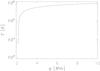 |
Fig. 1 Hydrostatic solar atmospheric temperature vs. height y. |
We adopt a realistic plasma temperature profile given by the semi-empirical model of Avrett & Loeser (2008) that is extrapolated into the solar corona (Fig. 1). In this model, the temperature attains a value of about 7 × 10³ K at the top of the chromosphere, y ≈ 2.0 Mm. At the transition region, which is located at y ≃ 2.1 Mm, T exhibits an abrupt jump (Fig. 1), and it grows to about 0.8 × 10⁶ K in the solar corona at y = 10 Mm. Higher up in the solar corona, the temperature increases very slowly, tending to its asymptotical value of about 1.6 MK. The temperature profile uniquely determines the equilibrium mass density and gas pressure profiles, which fall off with height (not shown).
2.2.2. Magnetohydrostatic equilibrium
Multiplying Eq. (5) by B, we obtain  (10)The solenoidal condition of Eq. (6) is automatically satisfied if we express the equilibrium magnetic field with the use of magnetic flux function A(x,y) as
  (11)where ez is a unit vector along z-direction, and Bz is the z-component of the magnetic field. We therefore have
 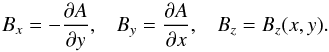 (12)We set
 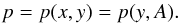 (13)Then from Eq. (10) we get
 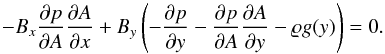 (14)With the use of Eq. (12), we simplify this equation to the hydrostatic condition along the magnetic field line, which is specified by the equation A = const.
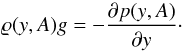 (15)We can express the x-, y-, and z-components of Eq. (5) as
![\begin{eqnarray} &&\frac{1}{\mu}\left[ B_{y}\left(\frac{\partial B_{x}}{\partial y} - \frac{\partial B_{y}}{\partial x} \right) - B_{z} \frac{\partial B_{z}}{\partial x} \right] = B_{y} \frac{\partial p}{\partial A}, \label{eq:EqS8} \\ &&\frac{1}{\mu} \left[ -B_{z} \frac{\partial B_{z}}{\partial y} \!-\!B_{x} \left( \frac{\partial B_{x}}{\partial y} \!-\! \frac{\partial B_{y}}{\partial x} \right)\right]\! =\! \frac{\partial p}{\partial y} \!+\! \frac{\partial p}{\partial A}\! \cdot\! \frac{\partial A}{\partial y} \!+\! \varrho (y)g\! =\! - B_{x} \frac{\partial p}{\partial A},\notag\\&& \label{eq:EqS10} \\ &&B_{y}\frac{\partial B_{z}}{\partial y}+ B_{x}\frac{\partial B_{z}}{\partial x} = J\left( \frac{A,B_{z}}{x,y}\right) = 0, \label{eq:EqS9} \end{eqnarray}](/articles/aa/full_html/2015/05/aa24601-14/aa24601-14-eq50.png)
where J() is the Jacobian. From the last equation it follows that 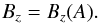 (19)Multiplying Eq. (16) by Bx and Eq. (17) by By and taking their sum, we obtain the equilibrium equation for a system with translational symmetry (Low 1975; Priest 1982):
 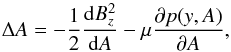 (20)where
  is the Laplacian. This equation, Eqs. (14), (15), and the equation of ideal gas comprise the system of equations of magnetohydrostatics.
We consider the inverse problem of magnetohydrostatics (Low 1980, 1982; Solov’ev 2010; Shapovalov & Shapovalova 2003), assuming that the flux function A(x,y) is known, and find the corresponding expressions for ϱ and p. Guided by this, we integrate Eq. (20) over A from infinity, where A = 0, p = ph(y) and the external field Bz(0) = Bz,ex = const., to some point of the configuration, and keep the coordinate y as a fixed parameter. As a result we get (see also Solov’ev 2010) 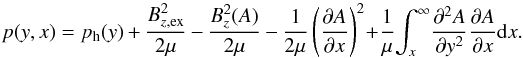 (21)When the external field Bz,ex is large enough, which may be the case for an active region, we can maintain a strong magnetic field in equilibrium thanks to the second positive term on the righthand side of Eq. (21).
To calculate the equilibrium mass density, we have to find ∂p(y,A) /∂y. For any differentiable function S(x,y), we satisfy the following relations:
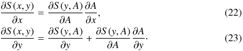
We calculate the derivative ∂S(y,A) /∂A taking into account that in our case S(x,y) = p(x,y). We rewrite Eq. (20) as 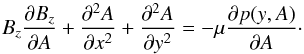 (24)From Eq. (23) we find
 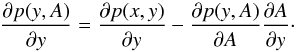 (25)Using this expression in Eq. (24), we get
 ![\begin{eqnarray} \frac{\partial p(y,A)}{\partial y} &=& \frac{\partial p_{\rm h}(y)}{\partial y}\, \nonumber\\ &&\quad\quad-\frac{1}{\mu}B_{z}\frac{\partial B_{z}}{\partial A}\frac{\partial A}{\partial y} -\frac{\partial}{\partial y}\left[ \frac{1}{2 \mu} \left( \frac{\partial A}{\partial x}\right) ^{2} - \frac{1}{\mu} \int^{\infty}_{x}\frac{\partial ^{2}A}{\partial y^{2}} \frac{\partial A}{\partial x} {\rm d}x \right] \nonumber\\ &&\quad\quad\quad\quad+ \frac{1}{\mu} B_{z} \frac{\partial B_{z}}{\partial A}\frac{\partial A}{\partial y}+\frac{1}{\mu} \Delta A \frac{\partial A}{\partial y}\cdot \label{eq:EqS19} \end{eqnarray}](/articles/aa/full_html/2015/05/aa24601-14/aa24601-14-eq71.png) (26)With the use of Eqs. (15) and (26), we obtain
(26)With the use of Eqs. (15) and (26), we obtain ![\begin{equation} \varrho (x,y) = \varrho_{\rm h}(y)+\frac{1}{2 \mu g} \frac{\partial}{\partial y} \left[ \left( \frac{\partial A}{\partial x}\right)^{2} - 2 \int^{\infty}_{x} \frac{\partial ^{2}A}{\partial y^{2}}\frac{\partial A}{\partial x} {\rm d}x \right] -\frac{1}{\mu} \frac{\partial A}{\partial y} \Delta A. \label{eq:EqS20} \end{equation}](/articles/aa/full_html/2015/05/aa24601-14/aa24601-14-eq72.png) (27)Equations (21) and (27) comprise the solution to the problem. They are valid for any choice of magnetic field that is determined by the magnetic flux function A(x,y) and transversal component Bz(A). The only condition is that the equilibrium gas pressure and mass density, given respectively by Eqs. (21) and (27), must be positive.
(27)Equations (21) and (27) comprise the solution to the problem. They are valid for any choice of magnetic field that is determined by the magnetic flux function A(x,y) and transversal component Bz(A). The only condition is that the equilibrium gas pressure and mass density, given respectively by Eqs. (21) and (27), must be positive.
2.2.3. The magnetic null line
Consider now the transversal magnetic-free case, Bz(A) = 0. From Eqs. (21) and (27), it follows that the equilibrium mass density, ϱ, and a gas pressure, p, simplify to the following expressions (see also Solov’ev 2010; Kraśkiewicz et al. 2015):
![\begin{eqnarray} &&\varrho(x,y) = \varrho_{\rm h}(y) \!+ \!\frac{1}{\mu g} \left[ \frac{\partial}{\partial y} \left(\! \int_{\rm \infty}^{x}\!\! \frac{\partial ^{2} A}{\partial y^{2}} \frac{\partial A}{\partial x} {\rm d}x \!+\! \frac{1}{2}\! \left(\frac{\partial A}{\partial x}\right)^{2} \right)\! -\! \frac{\partial A}{\partial y} \nabla ^{2} A \right] ,\notag\\&& \label{eq:B3} \\ &&\mu p(x,y) = \mu p_{\rm h}(y) -\frac{1}{2} \left(\frac{\partial A}{\partial x}\right)^{2} - \int_{\rm \infty}^{x} \frac{\partial ^{2} A}{\partial y^{2}} \frac{\partial A}{\partial x} {\rm d}x . \label{eq:B2} \end{eqnarray}](/articles/aa/full_html/2015/05/aa24601-14/aa24601-14-eq75.png)
For the solar magnetic null line, we choose the magnetic flux function as ![\begin{equation} \ A(x,y) = \frac{B_{0}}{k}\left[k x\, {\rm e} ^{-k^{2}x^{2}} {\rm e}^{-k(y - y_{\rm r})}+ a{kx}\right] , \label{eq:B4} \end{equation}](/articles/aa/full_html/2015/05/aa24601-14/aa24601-14-eq76.png) (30)where k is the inverse scale length, yr the vertical coordinate of the null line, and a = const. is a dimensionless parameter that is associated with the external magnetic field along the y-direction, which is specified as
(30)where k is the inverse scale length, yr the vertical coordinate of the null line, and a = const. is a dimensionless parameter that is associated with the external magnetic field along the y-direction, which is specified as  (31)Here ey is a unit vector along the y-direction. We set k = 1/3, a = − 0.75, and hold them fixed. Since a magnetic flux function, A(x,y), can be chosen arbitrarily, we set it in the form of Eqs. (30), (31). As for a< 0, it corresponds to two arcades that emerged from lower atmospheric layers into an originally vertical magnetic field, creating the null line above these arcades. It is noteworthy that any choice of A(x,y) corresponds to an equilibrium.
 |
Fig. 2 Equilibrium magnetic field lines. The magnetic null line is located at (x = 0, y ≅ 4.2) Mm. |
Magnetic field lines resulting from Eq. (30) are illustrated in Fig. 2. We note the presence of the null line located at (x = 0, y ≅ 4.2) Mm, where the magnetic field is zero. Below this point, close to the line x = 0 Mm, the magnetic field is essentially vertical, and it points downward. However, farther out from the line x = 0, the magnetic field lines reveal their curved nature. Above the null line, magnetic field lines are directed upward, and they are less curved than below the null line, which have the inverted Y-shape.
In this system the Alfvén speed, cA, varies along both the x- and y-directions, and it is expressed as  (32)where B is evaluated from Eq. (11) with Bz = 0 and the use of Eq. (30). The profile of log cA is displayed in Fig. 3 (top). The Alfvén speed is non-isotropic; highest values of cA are located at the places where the plasma is hottest (not shown), which is at the points (x = ± 2,y = 3) Mm. We specify the plasma β as the ratio of gas-to-magnetic pressures,
  (33)The spatial profiles of log β are illustrated in Fig. 3 (bottom). As B = 0 at the null line, β is infinitely large there. But it falls off with distance away from the null line.
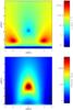 |
Fig. 3 Spatial profiles of cA(x,y) (top) and β(x,y) (bottom). |
 |
Fig. 4 Numerical blocks used in the numerical simulations. |
3. Numerical simulations of MHD equations
To solve Eqs. (1)−(3) numerically, we use the FLASH code (Fryxell et al. 2000; Lee & Deane 2009; Lee 2013), in which a third-order unsplit Godunov-type solver with various slope limiters and Riemann solvers, as well as adaptive mesh refinement (AMR; MacNeice et al. 1999), are implemented. The minmod slope limiter and the Roe Riemann solver (e.g., Tóth 2000) are used. We set the simulation box as (−3 Mm,3 Mm) × (1.9 Mm,7.9 Mm), while all plasma quantities remain invariant along the z-direction; however, both Vz and Bz generally differ from zero.
In our present work, we use an AMR grid with a minimum (maximum) level of refinement set to 3 (6). We performed the grid convergence studies by refining the grid by a factor of two. Because the numerical results remained essentially same for the grid of maximum block levels 6 and 7, we adopted the former to get the results presented in this paper. Small-size blocks of the numerical grid occupy the altitude of up to y ≈ 5.1 Mm, which is about 3 Mm above the solar transition region (Fig. 4), and every numerical block consists of 8 × 8 identical numerical cells. This results in an excellent resolution of steep spatial profiles and greatly reduces the numerical diffusion in these regions.
3.1. Shearing of magnetic field lines
At all four boundaries, we set all plasma quantities to their equilibrium values. The only exception is the bottom boundary, where we additionally place the shearing of magnetic field, described by  (34)Here Ad is the amplitude of the shearing, (0,y0) is its position, w denotes its width, and τB is the growth time of the shearing. We set and hold y0 = 1.9 Mm, w = 100 km, and τB = 100 s fixed, allowing Ad to vary. The value of y0 corresponds to the magnetic shearing working about 200 km below the transition region. The width w = 100 km mimics a localized source of the shearing. The implemented value of the growth time models a fast shearing, while long-lasting (over hours) shearings would be more realistic. However, such shearings would be expensive for numerical modelling, and therefore they are devoted for potential future studies.
4. Results of numerical simulations
Without shearing (Ad = 0) in our 2.5D model with the transverse magnetic-free case, Bz(A) = 0, the Alfvén waves would decouple from magnetoacoustic waves, and the Alfvén waves would be described solely by Vz(x,y,t) and Bz(x,y,t). As a result, Alfvén waves in the linear, one-dimensional limit would be approximately governed by the following wave equation:  (35)where l is the coordinate along a magnetic field line.
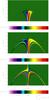 |
Fig. 5 Temporal evolution of Vz(x,y) for Ad = 2.28 Gauss at t = 200 s, t = 600 s, and t = 2 × 10³ s (from top to bottom). Arrows represent velocity vectors in the x-y plane, [ Vx, Vy ], expressed in the units of 0.1 km s-1. (Movie available online.) |
Figure 5 shows the spatial profiles of Vz(x,y) at three instants of time. A part of the simulation region is only displayed. Since the Alfvén speed is zero at the magnetic null line, the Alfvén waves are not able to reach this point. At t = 200 s, Alfvén waves propagate upward, approaching the null line (the top panel). As the magnetic field lines diverge with height, Alfvén waves follow them by turning in the left and right directions in the left (x< 0 Mm) and right (x> 0 Mm) half planes, respectively. This is seen at later moments of time (the middle and bottom panels). However, the Alfvén speed is highly inhomogeneous along magnetic field lines (Fig. 3). As a result of this inhomogeneity, the Alfvén waves experience scattering. However, the shearing of magnetic lines results in linear coupling between Alfvén and magnetoacoustic waves (e.g., Wołoszkiewicz et al. 2014), and although Vz corresponds essentially to Alfvén waves, it is also associated with fast magnetoacoustic waves. The latter are able to propagate across the null line, where as a result of disappearing magnetic field, they temporarily become acoustic waves. They enter the coronal region above the magnetic null line, which is clearly seen at t = 2 × 10³ s (bottom).
Figure 5 illustrates the velocity vectors [ Vx, Vy ] that at the initial stage of the system’s evolution, correspond to magnetoacoustic waves. At t = 200 s, two eddies appear at (x ≅ ± 0.5, y ≅ 3.2) Mm. At a later time, the flow in the x − y plane is more complex, but since it follows magnetic field lines, it is essentially associated with slow magnetoacoustic waves.
Figure 6 shows the evolution in time of Vz(x = 0.05 Mm, y) above the null line. The maximum of the absolute value of Vz(x = 0.05 Mm, y) increases in time, which proves that the wave signal indeed penetrates the coronal region above the null line.
As different parts of Alfvén waves move along magnetic field lines of different lengths, along which Alfvén speed varies differently, Alfvén waves experience phase-mixing (Fig. 5 middle and bottom) which is further illustrated in Fig. 7, which illustrates vertical profiles of Vz(x = 0.5 Mm, y) at t = 500 s, t = 600 s, and t = 103 s. At t = 500 s, the oscillations at y ≈ 3.3 Mm are approximately in anti-phase to the oscillations at the later moments of time, which reveal a high level of complexity, resulting from phase mixing and wave scattering.
Figure 8 clearly shows that the oscillations are present in the time signature of Vz collected at the point (x = 0.5, y = 3.5) Mm. The Fourier waveperiod of these oscillations, P, is about 333 s, which is close to the waveperiod of 5-min oscillations. However, P depends on a number of plasma quantities, such as a length of magnetic line and a profile of Alfvén speed along this line. These oscillations result essentially from partial reflection of Alfvén waves from the inhomogeneous region of high Alfvén speed located at (x = 1.9, y = 2.9) Mm (Fig. 3, bottom), and they decay in time as exp( − t/τ) (Fig. 8), where τ is a decaying time. The envelopes fit to the time signature (Fig. 8) show that for Ad = 2.28 Gauss, τ is approximately 362 s, which is only about 30 s longer than the waveperiod. As a result we infer that Alfvén waves are attenuated on time scales that are comparable to their waveperiod.
The transmission coefficient of the Alfvén waves signal through the transition region can be evaluated as  (36)where Ai = 2.2 km s-1 and At = 0.7 km s-1 are amplitudes of respectively incident (Fig. 9) and transmitted Alfvén waves (Fig. 9). As a result we get Ct ≈ 0.3. Because the reflection coefficient is Cr = 1 − Ct, we find that Cr ≈ 0.7, which means that about 70% of the waves amplitude became reflected from the transition region, and about 30% was transmitted into lower atmospheric layers. This rather high value of Ct means that Alfvén waves are strongly attenuated by a significant amount of Alfvén waves energy that is transmitted through the transition region into lower regions of the solar atmosphere.
Figure 10 shows a dependence of τ/P on Ad. A lower value of τ/P corresponds to stronger attenuation and τ/P attains a value of about 1.95 for Ad = 1.1 Gauss. For a bit higher values of Ad, τ/P falls off with Ad, attaining its minimum of about 1.05 at Ad = 2.2 Gauss. This behavior fulflils our expectations; for a higher value of Ad, we would expect that more magnetoacoustic waves are present in the system because Alfvén waves are strongly coupled to these waves owing to the presence of the sheared magnetic field. Indeed, Fig. 11 illustrates the ratio of kinetic energies of magnetoacoustic and Alfvén waves Ekm/EkA vs. Ad. The kinetic energy of magnetoacoustic waves increases with Ad. Figure 12 shows the evolution of the ratio of the total kinetic energy to the total magnetic energy in time. This ratio grows in time reaching its maximum of about 8.5 × 10⁻³ at t ≈ 1400 s and then, as the fast magnetoacoustic waves leave the simulation region, it subsides in time.
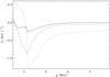 |
Fig. 6 Evolution of Vz(x = 0.05 Mm, y) above the null line at t = 103 s (solid line), t = 1.6 × 10³ s (dashed line), and t = 5 × 10³ s (dotted line) for Ad = 2.28 Gauss. |
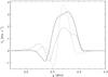 |
Fig. 7 Evolution of Vz(x = 0.5 Mm, y) at t = 500 s (solid line), t = 600 s (dashed line), and t = 103 s (dotted line) for Ad = 2.28 Gauss. |
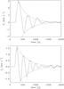 |
Fig. 8 Time history of Vz(x = 0.5 Mm, y = 3.5 Mm) (solid line) and its envelope (dashed lines) for Ad = 2.28 Gauss (top) and of Vz(x = 0.6 Mm, y = 3.3 Mm) and its envelope for Ad = 5.7 Gauss (bottom). |
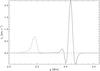 |
Fig. 9 Vertical profiles of Vz(x = 1.7 Mm, y) (solid line) and Vz(x = 2.2 Mm, y) (dashed line) at t = 103 s for Ad = 2.28 Gauss. |
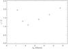 |
Fig. 10 Ratio of the attenuation time over wave period, τ/P, vs. the amplitude of the shearing, Ad. |
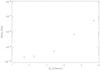 |
Fig. 11 Ratio of the kinetic energy of magnetoacoustic waves, Ekm, to the kinetic energy of Alfvén waves, EkA, within the simulation region at t = 103 s vs. the amplitude of the shearing, Ad. |
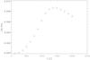 |
Fig. 12 Ratio of the total kinetic energy, Ek, to the the total magnetic energy, Em, within the simulation region vs. time t for Ad = 2.28 Gauss. |
From Fig. 10 we infer that for Ad> 2 Gauss τ/P grows with Ad. While P decreases slightly with Ad (not shown), a larger amplitude of the shearing results in less attenuation, which results from a prevalence of relaxation process over wave propagation, for which τ is larger. As a result, τ/P grows with Ad for Ad> 2.2 Gauss (Fig. 10).
The attenuation time also varies with a characteristic growing time of the shearing, τB (see Eq. (34)). For a higher value of τB, thereare supposed to be fewer oscillations, because the system essentially relaxes to a new quasi-equilibrium. That results in a higher value of τ. This effect is presented in Fig. 13. For τB = 200 s, we get τ ≃ 5.5 × 10³ s, while τB = 400 s corresponds to τ ≃ 12 × 103 s.
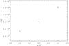 |
Fig. 13 Attenuation time, τ, vs. time of shearing τB. |
It is noteworthy that in many cases when shearing perturbations are applied in the vicinity of nulls, significant dissipation and perhaps reconnection occurs around the null/separatrices (e.g., Hassam & Lambert 1996; Craig & McClymont 1997; Antiochos & Linton 2002; Galsgaard et al. 2003; Craig & Litvinenko 2005; Pontin & Galsgaard 2007). However, the grid refinement studies that we performed showed that such phenomena are absent around the null line in our system.
5. Summary and conclusions
It is important to investigate the role of Alfvén waves on some solar phenomena, particularly when they are associated with the coronal heating and solar wind acceleration that remain long-standing problems of heliophysics. Leading into this framework, we generalized the analytical model of Kraśkiewicz et al. (2015) by implementing a magnetic field component along the invariant direction Bz. The model we devised can be adopted to derive equilibrium conditions for any 2.5D magnetic structure in the solar atmosphere. A magnetic field is specified by an arbitrary choice of a magnetic flux function A(x,y) and Bz(A). Having specified A(x,y), the equilibrium mass density and a gass pressure are expressed by Eqs. (21) and (27).
Using the devised analytical model of the magnetic null line, we performed the 2.5D numerical simulations of the shearing magnetic field lines, implemented about 200 km below the transition region. These simulations adapt the realistic model of the hydrostatic solar atmosphere in the FLASH code. Our model exhibits the formation of the Alfvén waves at the initial phase of temporal evolution, linear coupling between Alfvén and magnetoacoustic waves at a later time, and relaxation of the system in the final phase. Our results reveal the complex picture of interaction between Alfvén waves and magnetic null lines. We found that as a result of highly inhomogeneous Alfvén speed and different lengths of magnetic field lines, Alfvén waves experience phase mixing, scattering from inhomogeneous regions of Alfvén speed, and partial reflection from the transition region and other areas of highly varying Alfvén speed. As a consequence, Alfvén waves become attenuated with the attenuation time varying with the amplitude and characteristic time of the shearing. A larger shearing of magnetic field lines results in stronger linear coupling between Alfvén and magnetoacoustic waves. The kinetic energy of the latter waves increases with the amplitude of the shearing, but it remains lower than the kinetic energy of Alfvén waves (Fig. 11).
Online material
Movie of Fig. 5 Access here
Acknowledgments
The work was supported by a Marie Curie International Research Staff Exchange Scheme Fellowship within the 7th European Community Framework Program. A.S. thanks the Presidium of Russian Academy of Sciences for support in the frame of Program 9 and the Russian Foundation of Fundamental Research under the grant. The software used in this work was developed in part by the DOE-supported ASCI/Alliance Center for Astrophysical Thermonuclear Flashes at the University of Chicago. The visualizations of the simulation variables were carried out using the Interactive Data Language (IDL) software package.
References
- Antiochos, S. K., & Linton, M. G. 2002, ApJ, 581, 703 [NASA ADS] [CrossRef] [Google Scholar]
- Avrett, E. H., & Loeser, R. 2008, ApJS, 175, 228 [Google Scholar]
- Brown, D. S., & Priest, E. R. 2001, A&A, 367, 339 [NASA ADS] [CrossRef] [EDP Sciences] [Google Scholar]
- Bulanov, S. V., & Syrovatskii, S. I. 1980, Fiz. Plazmy., 6, 1205 [NASA ADS] [Google Scholar]
- Chmielewski, P., , & Murawski, K. 2014, ApJ, submitted [Google Scholar]
- Chmielewski, P., Srivastava, A. K., Murawski, K., & Musielak, Z. E. 2013, MNRAS, 428, 40 [NASA ADS] [CrossRef] [Google Scholar]
- Craig, I. J. D., & Litvinenko, Y. E. 2005, Phys. Plasmas, 12, 032301 [NASA ADS] [CrossRef] [Google Scholar]
- Craig, I. J. D., & McClymont, A. N. 1997, ApJ, 481, 996 [NASA ADS] [CrossRef] [Google Scholar]
- Fryxell, B., Olson, K., & Ricker, P. 2000, ApJS, 131, 273 [NASA ADS] [CrossRef] [Google Scholar]
- Fujimura, D., & Tsuneta, S. 2009, ApJ, 702, 1443 [NASA ADS] [CrossRef] [Google Scholar]
- Galsgaard, K., Priest, E. R., & Titov, V. S. 2003, J. Geophys. Res., 108, 1042 [NASA ADS] [CrossRef] [Google Scholar]
- Gruszecki, M., Murawski, K., Solanki, S., & Ofman, L. 2007, A&A, 469, 1117 [NASA ADS] [CrossRef] [EDP Sciences] [Google Scholar]
- Hassam, A. B., & Lambert, R. P. 1996, ApJ, 472, 832 [NASA ADS] [CrossRef] [Google Scholar]
- Jess, D. B., Mathioudakis, M., Erdélyi, R., et al. 2009, Science, 323, 1582 [NASA ADS] [CrossRef] [PubMed] [Google Scholar]
- Kraśkiewicz, J., Murawski, K., Solov’ev, A., & Srivastava, A. K. 2015, Sol. Phys., submitted [Google Scholar]
- Lee, D. 2013, J. Comput. Phys., 243, 269 [NASA ADS] [CrossRef] [Google Scholar]
- Lee, D., & Deane, A. E. 2009, J. Comput. Phys., 228, 952 [NASA ADS] [CrossRef] [Google Scholar]
- Low, B. C. 1975, ApJ, 197, 251 [NASA ADS] [CrossRef] [Google Scholar]
- Low, B. C. 1980, Sol. Phys., 65, 147 [NASA ADS] [CrossRef] [Google Scholar]
- Low, B. C. 1982, Sol. Phys., 75, 119 [Google Scholar]
- MacNeice, P., Spicer, D. S., & Antiochos, S. 1999, 8th SOHO Workshop: Plasma Dynamics and Diagnostics in the Solar Transition Region and Corona, ESA SP, 446, 457 [NASA ADS] [Google Scholar]
- McLaughlin, J. A., & Hood, A. W. 2004, A&A, 420, 1129 [NASA ADS] [CrossRef] [EDP Sciences] [Google Scholar]
- Murawski, K. 1992, Sol. Phys., 139, 279 [NASA ADS] [CrossRef] [Google Scholar]
- Murawski, K., & Musielak, Z. E. 2010, A&A, 518, A37 [NASA ADS] [CrossRef] [EDP Sciences] [Google Scholar]
- Musielak, Z. E., Routh, S., & Hammer, R. 2007, ApJ, 659, 650 [NASA ADS] [CrossRef] [Google Scholar]
- Nakariakov, V. M., & Verwichte, E. 2005, Liv. Rev. Sol. Phys., 2, 3 [Google Scholar]
- Nakariakov, V. M., Roberts, B., & Murawski, K. 1997, Sol. Phys., 175, 93 [NASA ADS] [CrossRef] [Google Scholar]
- Nakariakov, V. M., Roberts, B., & Murawski, K. 1998, A&A, 332, 795 [NASA ADS] [Google Scholar]
- Pontin, D. I., & Galsgaard, K. 2007, J. Geophys. Res., 112, 3103 [NASA ADS] [CrossRef] [Google Scholar]
- Priest, E. R. 1982, Solar magnetohydrodynamics (London: D. Reidel Publ. Comp.) [Google Scholar]
- Shapovalov, V. N., & Shapovalova, O. V. 2003, Izvestia Vuzov. Fisika., 46, 74 [Google Scholar]
- Solov’ev, A. 2010, Astron. Rep., 54, 85 [Google Scholar]
- Tóth, G. 2000, J. Comput. Phys., 161, 605 [Google Scholar]
- Van Doorsselaere, T., Nakariakov, V. M., & Verwichte, E. 2008, ApJ, 676, L73 [NASA ADS] [CrossRef] [Google Scholar]
- Vasheghani Farahani, S., Nakariakov, V. M., & Verwichte, E. 2012, A&A, 544, A127 [NASA ADS] [CrossRef] [EDP Sciences] [Google Scholar]
- Wołoszkiewicz, P., Murawski, K., Musielak, Z. E., & Mignone, A. 2014, Contr. Cyber., 43, 321 [Google Scholar]
- Zaqarashvili, T. V., & Murawski, K. 2007, A&A, 470, 353 [NASA ADS] [CrossRef] [EDP Sciences] [Google Scholar]
All Figures
|
Fig. 1 Hydrostatic solar atmospheric temperature vs. height y. |
| In the text | |
|
Fig. 2 Equilibrium magnetic field lines. The magnetic null line is located at (x = 0, y ≅ 4.2) Mm. |
| In the text | |
|
Fig. 3 Spatial profiles of cA(x,y) (top) and β(x,y) (bottom). |
| In the text | |
|
Fig. 4 Numerical blocks used in the numerical simulations. |
| In the text | |
|
Fig. 5 Temporal evolution of Vz(x,y) for Ad = 2.28 Gauss at t = 200 s, t = 600 s, and t = 2 × 10³ s (from top to bottom). Arrows represent velocity vectors in the x-y plane, [ Vx, Vy ], expressed in the units of 0.1 km s-1. (Movie available online.) |
| In the text | |
|
Fig. 6 Evolution of Vz(x = 0.05 Mm, y) above the null line at t = 103 s (solid line), t = 1.6 × 10³ s (dashed line), and t = 5 × 10³ s (dotted line) for Ad = 2.28 Gauss. |
| In the text | |
|
Fig. 7 Evolution of Vz(x = 0.5 Mm, y) at t = 500 s (solid line), t = 600 s (dashed line), and t = 103 s (dotted line) for Ad = 2.28 Gauss. |
| In the text | |
|
Fig. 8 Time history of Vz(x = 0.5 Mm, y = 3.5 Mm) (solid line) and its envelope (dashed lines) for Ad = 2.28 Gauss (top) and of Vz(x = 0.6 Mm, y = 3.3 Mm) and its envelope for Ad = 5.7 Gauss (bottom). |
| In the text | |
|
Fig. 9 Vertical profiles of Vz(x = 1.7 Mm, y) (solid line) and Vz(x = 2.2 Mm, y) (dashed line) at t = 103 s for Ad = 2.28 Gauss. |
| In the text | |
|
Fig. 10 Ratio of the attenuation time over wave period, τ/P, vs. the amplitude of the shearing, Ad. |
| In the text | |
|
Fig. 11 Ratio of the kinetic energy of magnetoacoustic waves, Ekm, to the kinetic energy of Alfvén waves, EkA, within the simulation region at t = 103 s vs. the amplitude of the shearing, Ad. |
| In the text | |
|
Fig. 12 Ratio of the total kinetic energy, Ek, to the the total magnetic energy, Em, within the simulation region vs. time t for Ad = 2.28 Gauss. |
| In the text | |
|
Fig. 13 Attenuation time, τ, vs. time of shearing τB. |
| In the text | |
Current usage metrics show cumulative count of Article Views (full-text article views including HTML views, PDF and ePub downloads, according to the available data) and Abstracts Views on Vision4Press platform.
Data correspond to usage on the plateform after 2015. The current usage metrics is available 48-96 hours after online publication and is updated daily on week days.
Initial download of the metrics may take a while.