© ESO, 2015

1. Introduction

Relativistic jets are surrounded by rich environments, and stars and dense medium inhomogeneities can enter into these jets leading to the formation of shocks, as considered for instance in Blandford & Koenigl (1979); Coleman & Bicknell (1985); Komissarov (1994); Bednarek & Protheroe (1997); Araudo et al. (2009, 2010, 2013); Barkov et al. (2010, 2012b); Perucho & Bosch-Ramon (2012), and Bosch-Ramon et al. (2012). These shocks are, only initially in some cases, almost standing shocks, at rest in the laboratory frame (LF). A similar situation can occur in the termination region of other relativistic outflows, such as pulsar winds in binary systems (Paredes-Fortuny et al. 2015).

In several previous papers that modelled the radiation from relativistic shocks at rest in the LF, the emitting region was circumscribed to the closest obstacle vicinity and, as the flow there is only mildly relativistic, the radiation Doppler boosting was not considered. However, there could be more jet energy available for non-thermal particles than assumed in these works, as the effective interaction area may be much larger than just the obstacle section. In addition to that, the flow initially moves at ≈c/ 3 right after the shock, and then is quickly accelerated further downstream because of strong pressure gradients. This effect is seen for instance in Fig. 2 in Bosch-Ramon et al. (2012). Therefore, even relatively close to the obstacle at rest, the shocked flow velocity is high enough for Doppler boosting to significantly enhance radiation in the emitting fluid direction of motion. The motion of the shocked flow could be also considered for an obstacle that is itself accelerated by the jet ram pressure (e.g. Barkov et al. 2012a; Khangulyan et al. 2013), but this would require accounting for the complex dynamical evolution of the obstacle (see Bosch-Ramon et al. 2012, for hydrodynamical simulations predicting the obstacle disruption).

In this work, we study the kinetic-to-internal (possibly non-thermal) energy conversion, gamma-ray radiation efficiency, and Doppler boosting effects, in the shock and the shocked flow of a relativistic hydrodynamic jet interacting with an obstacle at rest. The obstacle could be a star or a cloud in the case of an extragalactic jet, or a stellar wind inhomogeneity in the case of a galactic microquasar jet. Since this is a relevant and illustrative case, we focus here on the case of a population of red giant stars (RG) interacting with the jet of an active galactic nucleus (AGN). We first characterize the non-thermal luminosity from the shocked jet region accounting for hydrodynamical information, and second we adopt a phenomenological description of the spatial distribution of the RG in the regions crossed by the jet as it goes through the galaxy. To compute the emission, we consider mainly inverse Compton (IC) scattering, assume that synchrotron radiation is a minor emission channel, and put special emphasis on the GeV–TeV range. Studies such as this are needed to characterize the non-thermal emission from interactions between stars and jets in AGN, which is important if the AGN gamma-ray radiation is to be understood (e.g. Barkov et al. 2012a; Khangulyan et al. 2013).

Concerning other types of sources, the characterization of the radiation properties from jet-obstacle interactions could also shed light on the main factors shaping jet variability at high energies in microquasars (e.g. Owocki et al. 2009), or the post-shock emission in pulsar-wind termination shocks in some binary systems (e.g. Bosch-Ramon 2013). Regarding jets with strong magnetic fields with polarity changes, it has been proposed that the interaction with obstacles may lead to magnetic reconnection and efficient non-thermal emission (see Bosch-Ramon 2012). This kind of interaction is very complex given the strong dynamical role of the magnetic field and its non-trivial topological properties and deserves a specific treatment, which is beyond the scope of this paper.

2. The jet-RG wind interaction

2.1. Physical scenario

The study presented here is based on the interaction of a jet with an RG surrounded by its dense and slow wind. The basic hydrodynamical ingredients of this study are: a highly relativistic, supersonic flow with parallel fluid lines on the scales of interest; a cold obstacle at rest; and a fraction of the internal energy downstream of the standing shock being in the form of non-thermal particles. The initial speed of the RG is taken to be ≪c if it is to be approximated as at rest, so the problem can be considered axisymmetric around an axis crossing the star and with the jet flow direction. In addition, the RG wind must have enough inertia to stand the jet impact while it penetrates into the jet, which can be expressed as ${\mathit{\rho }}_{\mathrm{rg}}{\mathit{v}}_{\mathrm{rg}}^{\mathrm{2}}\mathit{>}{\mathit{L}}_{\mathrm{j}}\mathit{/}\mathit{\pi }{\mathit{R}}_{\mathrm{j}}^{\mathrm{2}}\mathit{c}$, where ρ_rg and v_rg are the RG wind density and velocity perpendicular to the jet, and L_j and R_j are the jet power and radius, respectively. In addition, in the standing shock scenario the velocity acquired by the RG wind due to jet impact must be ≪c. If these conditions are fulfilled, the problem becomes two dimensional, and the steady state of the physical system can be taken as the steady state of the shocked jet flow, which significantly lightens the hydrodynamical calculations presented in what follows.

2.2. Simulations

The jet-RG wind interaction was simulated in 2D assuming axisymmetry. We solved the equations of relativistic hydrodynamics using a Marquina Riemann solver (Donat & Marquina 1996), second-order spatial reconstruction scheme (minbee slope limiter, plus an additional dissipation term from Colella 1985), and an adiabatic gas with index . The resolution is 600 cells in the vertical direction, the z-axis, and 300 in the radial direction, the r-axis, and the physical size is z_max = 2 × 10¹⁵ cm in the z-direction, and r_max = 10¹⁵ cm in the r-direction. The jet power injected in the grid is ≈10³⁷ erg s^-1, with a Lorentz factor γ_j = 10. We fix the RG wind radius to R_rg = 10¹⁴ cm. A snapshot of the density distribution in the steady state is presented in Fig. 1. The shocked jet material is clearly seen in light blue, forming a cometary tail pointing upwards and surrounding the RG wind, red with green borders.

For simplicity, we modelled the RG wind region as a sphere with a density 10⁸ times that of the jet in the FF. As the shocked RG wind is much slower than the shocked jet flow, we considered it static, and thus the steady state of the simulation is quickly reached. In a more realistic setup, there would be more wind momentum flux perpendicular to the jet direction, slightly widening the shocked flow structure, but this setup would have required a simulation ~10³ times longer.

We chose the grid resolution such that numerical viscosity played a negligible role in the generation of internal energy in the shocked flow. There is some mixing in the RG wind-shocked jet flow boundary, but it has a minor impact on the radiation estimates presented below. This mixing slows down the shocked jet flow close to the axis, reducing the effect of Doppler boosting and thus weakening the emission from those (small) regions.

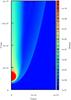Fig. 1 Distribution of density in the flow frame in cgs units.

For illustrative purposes, the simulation result is interpreted as an AGN jet of L_j ≈ 10⁴⁴ erg s^-1 and R_j = 1 pc, much larger than the grid, interacting with an RG wind region whose size is derived assuming jet-stellar wind pressure balance 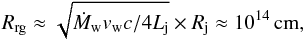${\mathit{R}}_{\mathrm{rg}}\mathrm{\approx }\sqrt{\mathit{Ṁ}\mathrm{w}{\mathit{v}}_{\mathrm{w}}\mathit{c}\mathit{/}\mathrm{4}{\mathit{L}}_{\mathrm{j}}}\mathrm{\times }{\mathit{R}}_{\mathrm{j}}\mathrm{\approx }{\mathrm{10}}^{\mathrm{14}}\hspace{0.17em}\mathrm{cm}\mathit{,}$(1)for a stellar mass loss Ṁ_w = 10^-8M_⊙/yr and a wind velocity v_w ≈ 2 × 10⁷ cm s^-1, typical of an RG. Note that for a real RG wind the actual size of the obstacle would be slightly larger than for the case of an obstacle of very large inertia, as the shocked wind region should be added in Eq. (1).

Relativistic jets usually present half semi-opening angles of several degrees, α_j ~ 0.1 rad, which for a supersonic jet without lateral causal contact yields γ_j = 1/α_j ~ 10 (see Khangulyan et al. 2013, and references therein). This condition implies an interaction height of z_j = γ_jR_j ~ 10 pc.

3. Non-thermal emission

We use the hydrodynamical information obtained in Sect. 2 to derive some important physical properties that allow for the characterization of the non-thermal emission. These properties are the radiative efficiency, the distribution of the non-thermal energy, the Doppler boosting, and the effective section of the RG wind as an obstacle for the jet.

3.1. Radiative efficiency and non-thermal energy distribution

To estimate the non-thermal emission, the radiative efficiency of the shocked flow is needed. This efficiency can be quantified as the radiative (1 /t_rad) to total (1 /t_c) cooling rate ratio (f_rad): ${\mathit{f}}_{\mathrm{rad}}\mathrm{=}{\mathit{t}}_{\mathrm{rad}}^{-1}\mathit{/}{\mathit{t}}_{\mathrm{c}}^{-1}\mathrm{=}{\mathit{t}}_{\mathrm{rad}}^{-1}\mathit{/}\mathrm{(}{\mathit{t}}_{\mathrm{rad}}^{-1}\mathrm{+}{\mathit{t}}_{\mathrm{nrad}}^{-1}\mathrm{)}\mathrm{=}\mathrm{(}\mathrm{1}\mathrm{+}{\mathit{t}}_{\mathrm{rad}}\mathit{/}{\mathit{t}}_{\mathrm{nrad}}{\mathrm{)}}^{-1}\mathit{,}$(2)where 1 /t_c also takes non-radiative cooling, 1 /t_nrad, into account. The timescale for non-radiative cooling, i.e. particle escape and adiabatic losses, is estimated in the flow frame (FF) as the distance between each point to the RG location (d_rg) divided by the local velocity (v_sh) times the shocked flow Lorentz factor (γ_sh): t_nrad = d_rg/v_shγ_sh. For the radiative timescale we adopt: t_rad = C_ICu^-1E^-1, where C_IC ≈ 26 in cgs units. This timescale is derived assuming IC in Thomson, and taking a reference electron energy of ${\mathit{E}}_{\mathrm{IC}}\mathrm{=}{\mathit{m}}_{\mathrm{e}}^{\mathrm{2}}{\mathit{c}}^{\mathrm{4}}\mathit{/}{\mathit{ϵ}}_{\mathrm{0}}$, where E_IC is roughly the energy of the IC cross-section maximum, and ϵ₀ is the target photon energy and u the energy density of a photon field coming from the RG, all in the FF. An effective stellar temperature of 3000 K has been taken, typical for an RG. The star luminosity, needed to obtain u, has been determined through ${\mathit{L}}_{\mathrm{\ast }}\mathrm{=}\mathit{Ṁ}{}_{\mathrm{w}}\mathit{v}_{\mathrm{w}}\mathit{c}$ (LF). This is a rather conservative assumption, as in fact only a fraction of all the star radiation momentum goes to the stellar wind. Note that protons are not taken into account as emitting particles.

Figure 2 shows the distribution of f_rad in the shocked flow. As seen in the figure, for the adopted jet and RG wind properties, f_rad is everywhere below one for the case simulated, i.e. the flow is adiabatic. In this case, the thermal pressure (P) of the shocked flow is a good proxy for the non-thermal energy distribution, which can be taken to be proportional to P all through the shocked flow. In Fig. 3, the distribution of P in the shocked flow is shown in a colour scale, from red to light green.

The characterization of the radiative and the non-radiative timescales, and of the non-thermal energy distribution, allows for the computation of an approximate total luminosity for IC in the FF, L_IC, simplifying the IC emissivity as that at E_IC. For moderately magnetized shocked flows, the synchrotron luminosity L_sync may be higher than L_IC, as ${\mathit{L}}_{\mathrm{sync}}\mathrm{\propto }{\mathit{E}}_{\max }^{\mathrm{3}\mathrm{-}\mathit{\alpha }}$, where α is the power-law index of the particle energy distribution, and E_max is the maximum electron energy, which could be ≫ E_IC. Under efficient particle acceleration and γ_j ≳ 10, the synchrotron spectrum may contribute to or dominate in the gamma-ray band. However, as the magnetic field is not well constrained, we will assume here that the synchrotron component can be neglected.

The adopted radiation cooling model is simple, although it accounts for the basic IC cross-section properties, and the target density behaviour under relativistic motion of the emitter. Therefore, the model should yield reasonable luminosity predictions for IC gamma rays, if gamma-ray pair-creation absorption is negligible.

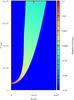Fig. 2 Distribution of radiation efficiency for the shocked jet region.

3.2. Doppler boosting and obstacle effective radius

The radiation enhancement due to Doppler boosting is ${\mathit{\delta }}_{\mathrm{sh}}^{\mathrm{4}}\mathrm{=}\mathrm{1}\mathit{/}{\mathit{\gamma }}_{\mathrm{sh}}^{\mathrm{4}}\mathrm{(}\mathrm{1}\mathrm{-}\cos {\mathit{\theta }}_{\mathrm{sh}}{\mathit{\beta }}_{\mathrm{sh}}{\mathrm{)}}^{\mathrm{4}}\mathit{,}$(3)which can be approximated as ≈$\mathrm{16}{\mathit{\gamma }}_{\mathrm{sh}}^{\mathrm{4}}$ when the angle between the jet and the observer directions is θ_obs ≪ 1 /γ_sh.

Figure 4 shows the distribution of the factor of enhancement of the emission from the shocked flow because of Doppler boosting. As seen in Fig. 4, values of ${\mathit{\delta }}_{\mathrm{sh}}^{\mathrm{4}}$ of a few are found right after the shock, but further downstream ${\mathit{\delta }}_{\mathrm{sh}}^{\mathrm{4}}$ achieves values as high as several thousand.

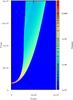Fig. 3 Distribution of pressure in cgs units for the shocked jet region.

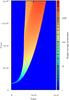Fig. 4 Distribution of the Doppler boosting enhancement (${\mathit{\delta }}_{\mathrm{sh}}^{\mathrm{4}}$) for the shocked jet region.

Another important result from our simulation is derived when computing , the rate of the total thermal energy generated in the interaction region in the LF, where the total thermal energy is the sum of internal energy plus the pressure component. The value of has been computed as the fraction of L_j that escapes the grid in the form of thermal energy. From this, we can derive the effective radius (R_eff) of the RG wind when acting as an obstacle for the jet $\mathit{U̇}\mathrm{sh}\mathrm{=}\mathrm{(}{\mathit{R}}_{\mathrm{eff}}\mathit{/}{\mathit{R}}_{\mathrm{j}}{\mathrm{)}}^{\mathrm{2}}{\mathit{L}}_{\mathrm{j}}\mathrm{\approx }\mathrm{4}\mathrm{\times }{\mathrm{10}}^{\mathrm{36}}\hspace{0.17em}{\mathrm{erg}\mathrm{s}}^{-1}\mathit{,}$(4)which turns out to be R_eff ≈ 6 R_rg because of effective kinetic to internal energy conversion even in regions far from the RG. This effective conversion manifests itself locally as well, as shown by Fig. 5.

The value of R_eff is actually dependent on R_rg and z_max. To check this dependence, two additional simulations were carried out, both with twice the cell size of the presented simulation, one with the same grid size, and the other with a grid that is twice as large, and both with the same remaining parameters. These simulations show that R_eff grows slowly with r_max. This is expected to happen as the oblique shock becomes weaker farther away from the RG, but the actual weakening of the shock is sensitive to the specific value of the unshocked flow internal energy, which is unknown. Note also that to derive R_eff all the grid is taken into account; in reality, the efficiency of energy conversion is larger if the grid outermost region without shock presence is neglected. Therefore, R_eff = 6 R_rg may be considered a lower limit.

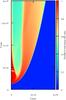Fig. 5 Distribution of the ratio of fluxes of thermal energy to kinetic plus thermal energy.

4. The IC luminosity from a jet-obstacle interaction

4.1. The IC luminosity to the observer

Using the hydrodynamics results and under the simplified emission model described, we can derive an approximate observer IC luminosity of the shocked flow within the grid from 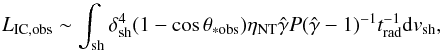${\mathit{L}}_{\mathrm{IC}\mathit{,}\mathrm{obs}}\mathrm{~}{\mathrm{\int }}_{\mathrm{sh}}{\mathit{\delta }}_{\mathrm{sh}}^{\mathrm{4}}\mathrm{(}\mathrm{1}\mathrm{-}\cos {\mathit{\theta }}_{\mathrm{\ast }\mathrm{obs}}\mathrm{)}{\mathit{\eta }}_{\mathrm{NT}}\mathit{\gamma ̂}\mathit{P}\mathrm{(}\mathit{\gamma ̂}\mathrm{-}\mathrm{1}{\mathrm{)}}^{-1}{\mathit{t}}_{\mathrm{rad}}^{-1}\mathrm{d}{\mathit{v}}_{\mathrm{sh}}\mathit{,}$(5)where dv_sh is the shocked flow differential volume, and θ_{∗ obs} the angle between the stellar photons and the observer direction, both in the FF. The term (1 − cosθ_{∗ obs}) is a term related to the IC scattering probability-dependence on the stellar photon and observer directions. The quantity η_NT is the ratio of non-thermal to total thermal energy density; it is a free parameter of value between 0 and 1. For a typical accelerated electron population, say with a particle energy distribution harder than ∝E^-3, given the value of ϵ₀, and accounting for Doppler boosting, the IC radiation will be mostly radiated in the GeV–TeV range, as seen by the observer.

From Eq. (5), the total observer IC luminosity is computed, obtaining L_IC,obs ~ 10³⁵η_NT erg s^-1, which is ≈ 1 η_NT% of the jet luminosity injected in the grid, and a ≈3 η_NT% of . On the other hand, neglecting relativistic effects and confining the emitter to the RG wind vicinity, one would get L_IC,obs ~ 3 × 10³²η_NT erg s^-1, which is ~300 times smaller than the more realistic value. This shows that the radiation can be underestimated if the interaction region is not globally taken into account.

Figure 6 shows the structure of the observer IC emitter for θ_obs ≪ 1 /γ_sh, produced in ring-like cells of volume 2πr_jΔr_jΔz_j, where Δr_j = r_max/ 300 and Δz_j = z_max/ 600. As seen in the figure, most of the emission comes from the closest regions to the RG, but also from farther away, close to the jet shock.

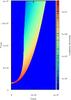Fig. 6 Distribution of the observer IC luminosity in cgs units for the shocked jet region.

4.2. Generalization of the results

For the adopted approximation z_j ~ γ_jR_j, our results correspond to an emitter located at relatively high heights (~10 pc) in a jet of moderate power (~10⁴⁴ erg s^-1). These results can nevertheless be generalized through 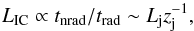${\mathit{L}}_{\mathrm{IC}}\mathrm{\propto }{\mathit{t}}_{\mathrm{nrad}}\mathit{/}{\mathit{t}}_{\mathrm{rad}}\mathrm{~}{\mathit{L}}_{\mathrm{j}}{\mathit{z}}_{\mathrm{j}}^{-1}\mathit{,}$(6)so L_IC,obs will grow closer to the jet base and/or with a more powerful jet. In saturation, Eq. (6) is not valid anymore as t_rad → t_nrad, and thus Eq. (5) becomes ${\mathit{L}}_{\mathrm{IC}\mathit{,}\mathrm{obs}}^{\max }\mathrm{~}{\mathrm{10}}^{\mathrm{2}}{\mathit{\eta }}_{\mathrm{NT}}\mathit{U̇}\mathrm{sh}\mathrm{\approx }\mathrm{4}\mathrm{\times }{\mathrm{10}}^{\mathrm{38}}{\mathit{\eta }}_{\mathrm{NT}}\hspace{0.17em}{\mathrm{erg}\mathrm{s}}^{-1}\mathit{,}$(7)i.e. it gets constant, for the same remaining parameters: γ_j and Ṁv_w.

The value of L_IC,obs is also ∝${\mathit{\gamma }}_{\mathrm{j}}^{\mathrm{2}}$, for θ_obs ≪ 1 /γ_sh and γ_j,sh ≫ 1. This relation comes from the relation γ_sh ∝ γ_j, strictly valid in the highly relativistic case, and the link between the IC luminosity in the LF (L_IC,lab) and L_IC,obs: ${\mathit{L}}_{\mathrm{IC}\mathit{,}\mathrm{obs}}\mathit{/}{\mathit{L}}_{\mathrm{IC}\mathit{,}\mathrm{lab}}\mathrm{\propto }{\mathit{\delta }}_{\mathrm{sh}}^{\mathrm{4}}\mathit{/}{\mathit{\gamma }}_{\mathrm{sh}}^{\mathrm{2}}\mathrm{\approx }\mathrm{16}\hspace{0.17em}{\mathit{\gamma }}_{\mathrm{sh}}^{\mathrm{2}}\mathrm{\propto }{\mathit{\gamma }}_{\mathrm{j}}^{\mathrm{2}}\mathit{.}$(8)Therefore, the computed estimates can be analytically generalized through 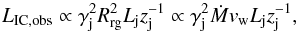${\mathit{L}}_{\mathrm{IC}\mathit{,}\mathrm{obs}}\mathrm{\propto }{\mathit{\gamma }}_{\mathrm{j}}^{\mathrm{2}}{\mathit{R}}_{\mathrm{rg}}^{\mathrm{2}}{\mathit{L}}_{\mathrm{j}}{\mathit{z}}_{\mathrm{j}}^{-1}\mathrm{\propto }{\mathit{\gamma }}_{\mathrm{j}}^{\mathrm{2}}\mathit{Ṁ}{\mathit{v}}_{\mathrm{w}}{\mathit{L}}_{\mathrm{j}}{\mathit{z}}_{\mathrm{j}}^{-1}\mathit{,}$(9)or in saturation, through 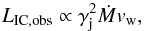${\mathit{L}}_{\mathrm{IC}\mathit{,}\mathrm{obs}}\mathrm{\propto }{\mathit{\gamma }}_{\mathrm{j}}^{\mathrm{2}}\mathit{Ṁ}{\mathit{v}}_{\mathrm{w}}\mathit{,}$(10)relations that also account for different types of winds via Ṁv_w.

For a microquasar jet, given the typical clump sizes (e.g. Owocki et al. 2009), clumps with R_eff ~ R_j may reach the jet. Also, IC emission may take place in saturation given the proximity of the stellar companion, yielding luminosities as high as${\mathit{L}}_{\mathrm{IC}\mathit{,}\mathrm{obs}}\mathrm{~}\mathrm{16}{\mathit{\gamma }}_{\mathrm{sh}}^{\mathrm{2}}{\mathit{\eta }}_{\mathrm{NT}}{\mathit{L}}_{\mathrm{j}}\mathit{,}$(11)which could be ≫ L_j for some relatively exceptional, and brief, events.

5. A population of red giants within an AGN jet

We explore in what follows whether collectively RG may be relevant for the non-thermal emission from AGN jets. About a 5% of the stars in the AGN vicinity are expected to be RG (Syer & Ulmer 1999). In addition, there are observational hints of stars interacting with AGN jets (e.g. Hardcastle et al. 2003; Müller et al. 2014). Therefore, the scenario explored in this work, and already postulated as the origin of high-energy emission by several authors (see Sect. 1), could be actually a rather common phenomenon.

We take the nearby, gamma-ray emitting AGN M87 as an example. With ~10¹¹ stars in the inner ~1 kpc of the galaxy (see Fig. 7 in Gebhardt & Thomas 2009), the number of RG within one jet should be about ${\mathit{N}}_{\mathrm{RG}}\mathrm{~}\mathrm{0.05}\mathrm{\times }{\mathrm{10}}^{\mathrm{11}}\mathrm{\times }\mathrm{3}{\mathit{\alpha }}_{\mathrm{j}}^{\mathrm{2}}\mathit{/}\mathrm{4}\mathrm{\approx }\mathrm{4}\mathrm{\times }{\mathrm{10}}^{\mathrm{7}}\mathit{,}$(12)where we take α_j ~ 0.1, and $\mathrm{3}{\mathit{\alpha }}_{\mathrm{j}}^{\mathrm{2}}\mathit{/}\mathrm{4}$ is the jet to total volume ratio.

Assuming an RG density ${\mathit{n}}_{\mathrm{RG}}\mathrm{\propto }\mathrm{1}\mathit{/}{\mathit{z}}_{\mathrm{j}}^{\mathit{\xi }}$, an average $\mathit{Ṁ}{}_{\mathrm{w}}\mathit{v}_{\mathrm{w}}\mathrm{~}{\mathrm{10}}^{\mathrm{25}}$ g cm s^-2, the relation from Eq. (6), negligible synchrotron radiation, a constant γ_j = 10, and L_j = 10⁴⁴ erg s^-1, each interaction would produce in gamma rays ${\mathit{L}}_{\mathrm{IC}\mathit{,}\mathrm{obs}}\mathrm{\left(}{\mathit{z}}_{\mathrm{j}}\mathrm{\right)}\mathrm{~}{\mathit{L}}_{\mathrm{IC}\mathit{,}\mathrm{obs}}\mathrm{\left(}{\mathit{z}}_{\min }\mathrm{\right)}\mathrm{\times }\mathrm{(}{\mathit{z}}_{\min }\mathit{/}{\mathit{z}}_{\mathrm{j}}\mathrm{)}\mathit{,}$(13)where z_min ≈ 8 × 10¹⁵ cm is found through L_IC,obs(10 pc) = 10³⁵η_NT erg s^-1, and fixing the z_min-luminosity to the saturation value: ${\mathit{L}}_{\mathrm{IC}\mathit{,}\mathrm{obs}}\mathrm{\left(}{\mathit{z}}_{\min }\mathrm{\right)}\mathrm{=}{\mathit{L}}_{\mathrm{IC}\mathit{,}\mathrm{obs}}^{\max }$. All this allows us to derive $\begin{array}{ccc}{\mathit{L}}_{\mathrm{IC}\mathit{,}\mathrm{obs}}^{\mathrm{tot}}& \mathrm{=}& \\ & \mathrm{=}& {\mathit{N}}_{\mathrm{RG}}\left(\frac{\mathrm{3}\mathrm{-}\mathit{\xi }}{\mathrm{2}\mathrm{-}\mathit{\xi }}\right)\left(\frac{{\mathit{z}}_{\max }^{\mathrm{2}\mathrm{-}\mathit{\xi }}\mathrm{-}{\mathit{z}}_{\min }^{\mathrm{2}\mathrm{-}\mathit{\xi }}}{{\mathit{z}}_{\max }^{\mathrm{3}\mathrm{-}\mathit{\xi }}\mathrm{-}{\mathit{z}}_{\min }^{\mathrm{3}\mathrm{-}\mathit{\xi }}}\right){\mathit{L}}_{\mathrm{IC}\mathit{,}\mathrm{obs}}\mathrm{\left(}{\mathit{z}}_{\min }\mathrm{\right)}\mathrm{\times }{\mathit{z}}_{\min }\mathit{,}\end{array}$(14)where dv_j is the jet differential volume.

The dominant contribution to ${\mathit{L}}_{\mathrm{IC}\mathit{,}\mathrm{obs}}^{\mathrm{tot}}$ will come from the inner-jet regions, or from galactic scales, depending on whether ξ is > or < than 2. For ξ ≈ 2, the z_min,max-dependence of ${\mathit{L}}_{\mathrm{IC}\mathit{,}\mathrm{obs}}^{\mathrm{tot}}$ is weak, but the external jet regions dominate. For this ξ-value¹, Eq. (14) gives ${\mathit{L}}_{\mathrm{IC}\mathit{,}\mathrm{obs}}^{\max }\mathrm{~}\mathrm{5}\mathrm{\times }{\mathrm{10}}^{\mathrm{41}}{\mathit{\eta }}_{\mathrm{NT}}$ erg s^-1, implying that the contribution from all RG within 1 kpc could be up to a factor of a few above the persistent GeV–TeV luminosities in M87 (e.g. Abdo et al. 2009; Aleksić et al. 2012). It seems unlikely however that the acceleration efficiency will be η_NT ~ 1, and we may be overestimating the average value of Ṁv_w. On the other hand, we do not take into account the asymptotic giant branch (AGB) and massive star contribution, both of which should be added to that of RG. Non-stellar objects such as clouds could also be relevant. Finally, the value of L_∗ could be significantly higher, at least in some stars. In conclusion, ${\mathit{L}}_{\mathrm{IC}\mathit{,}\mathrm{obs}}^{\max }$ may explain the persistent GeV–TeV emission in M87, and could be significant for AGN jets in general.

Note that the viewing angle with respect to the M87 jet is not zero, but rather ~20° (e.g. Acciari et al. 2009). However, given the obtained values of γ_sh (≲4), an angle of 20° is small enough for the condition θ_obs ≪ 1 /γ_sh to marginally apply. Here, the gamma-ray luminosity for M87 has been computed using the proper viewing angle, although taking θ_obs = 0 yields very similar results.

6. Discussion

The emission coming from the jet in Blazar AGN will be more boosted than that from the downstream region of a standing shock. Thus, strong jet activity could mask the putative jet-obstacle emission. However, for slightly misaligned, relatively nearby AGN, or those without significant non-thermal activity intrinsic of the jet, the contribution from populations of stars interacting with the jet could be important, ~0.1−1% of L_j (but strongly dependent on η_NT, γ_j, and θ_obs). This collective emission should be constant unless ξ were significantly softer than 2, which does not seem realistic. There could also be rare flaring events when a dense cloud, an AGB, a Wolf-Rayet or a luminous blue variable (WR/LBV) star, entered into the jet close to its base (e.g. Araudo et al. 2010, 2013; Barkov et al. 2010; Hubbard & Blackman 2006). In the case of microquasar jets, the ratio R_eff/R_j can be larger than in the extragalactic case and fluctuations may be more common, with the arrival of larger clumps leading to brighter events (Owocki et al. 2009; Araudo et al. 2009). This may also happen in binary systems hosting a non-accreting pulsar (see Bosch-Ramon 2013; Paredes-Fortuny et al. 2015, and references therein).

The obtained numerical results have been used to characterize the effective section of the RG wind as an obstacle for the jet, the distribution of the non-thermal particles through the constant η_NT, and the effect of Doppler boosting in the shocked flow for γ_j ≫ 1. Previous research focussed on a region downstream of the jet shock next to the obstacle and with a similar size (e.g. Araudo et al. 2009, 2010; Barkov et al. 2010, 2012b, and Doppler boosting effects were not considered as the flow is mildly relativistic there. As shown here, both approximations can lead to the underestimation of the non-thermal emission from jet-obstacle interactions.

Our work has some caveats. The simulation, in axisymmetry, without thermal cooling nor magnetic field, with modest resolution, and with a simple prescription of the RG wind, is not very realistic, although it captures the basic features of the shocked region of a hydrodynamic jet. The value of f_rad is a rough characterization of the radiative efficiency for IC, and our model of the IC emission is very simplified: it assumes IC only in Thomson, and accounts only for the electron energy at the maximum of the IC cross section. This simplification introduces an uncertainty in the predicted luminosity by a factor of a few. On the other hand, our radiation calculations account for the main features of IC scattering, and so we expect our results to be correct within an order of magnitude. Note that the value η_NT cannot be derived from first principles, and despite η_NT ≳ 0.1 are not uncommon in relativistic jet sources, η_NT ≪ 1 are also possible. It is also difficult to constrain the magnetic field strength in jets, which affects the calculation of synchrotron radiation. More accurate calculations will be presented in future work.

Acknowledgments

V.B.-R. acknowledges support by the Spanish Ministerio de Economía y Competitividad (MINECO) under grant AYA2013-47447-C3-1-P. This research has been supported by the Marie Curie Career Integration Grant 321520. V.B-R. also acknowledges financial support from MINECO and European Social Funds through a Ramón y Cajal fellowship.

References

All Figures

	Fig. 1 Distribution of density in the flow frame in cgs units.
In the text

	Fig. 2 Distribution of radiation efficiency for the shocked jet region.
In the text

	Fig. 3 Distribution of pressure in cgs units for the shocked jet region.
In the text

	Fig. 4 Distribution of the Doppler boosting enhancement (${\mathit{\delta }}_{\mathrm{sh}}^{\mathrm{4}}$) for the shocked jet region.
In the text

	Fig. 5 Distribution of the ratio of fluxes of thermal energy to kinetic plus thermal energy.
In the text

	Fig. 6 Distribution of the observer IC luminosity in cgs units for the shocked jet region.
In the text

References

- Abdo, A. A., Ackermann, M., Ajello, M., et al. 2009, ApJ, 707, 55 [NASA ADS] [CrossRef] [Google Scholar]
- Acciari, V. A., Aliu, E., Arlen, T., et al. 2009, Science, 325, 444 [NASA ADS] [CrossRef] [PubMed] [Google Scholar]
- Aleksić, J., Alvarez, E. A., Antonelli, L. A., et al. 2012, A&A, 544, A96 [NASA ADS] [CrossRef] [EDP Sciences] [Google Scholar]
- Araudo, A. T., Bosch-Ramon, V., & Romero, G. E. 2009, A&A, 503, 673 [NASA ADS] [CrossRef] [EDP Sciences] [Google Scholar]
- Araudo, A. T., Bosch-Ramon, V., & Romero, G. E. 2010, A&A, 522, A97 [NASA ADS] [CrossRef] [EDP Sciences] [Google Scholar]
- Araudo, A. T., Bosch-Ramon, V., & Romero, G. E. 2013, MNRAS, 436, 3626 [NASA ADS] [CrossRef] [Google Scholar]
- Barkov, M. V., Aharonian, F. A., & Bosch-Ramon, V. 2010, ApJ, 724, 1517 [NASA ADS] [CrossRef] [Google Scholar]
- Barkov, M. V., Aharonian, F. A., Bogovalov, S. V., Kelner, S. R., & Khangulyan, D. 2012a, ApJ, 749, 119 [NASA ADS] [CrossRef] [Google Scholar]
- Barkov, M. V., Bosch-Ramon, V., & Aharonian, F. A. 2012b, ApJ, 755, 170 [NASA ADS] [CrossRef] [Google Scholar]
- Bednarek, W., & Protheroe, R. J. 1997, MNRAS, 287, L9 [NASA ADS] [CrossRef] [Google Scholar]
- Blandford, R. D., & Koenigl, A. 1979, Astrophys. Lett., 20, 15 [NASA ADS] [Google Scholar]
- Bosch-Ramon, V. 2012, A&A, 542, A125 [NASA ADS] [CrossRef] [EDP Sciences] [Google Scholar]
- Bosch-Ramon, V. 2013, A&A, 560, A32 [NASA ADS] [CrossRef] [EDP Sciences] [Google Scholar]
- Bosch-Ramon, V., Perucho, M., & Barkov, M. V. 2012, A&A, 539, A69 [NASA ADS] [CrossRef] [EDP Sciences] [Google Scholar]
- Colella, P. 1985, SIAM J. Sci. Stat. Comput., 6, 104 [CrossRef] [Google Scholar]
- Coleman, C. S., & Bicknell, G. V. 1985, MNRAS, 214, 337 [NASA ADS] [CrossRef] [Google Scholar]
- Donat, R., & Marquina, A. 1996, J. Comput. Phys., 125, 42 [NASA ADS] [CrossRef] [Google Scholar]
- Gebhardt, K., & Thomas, J. 2009, ApJ, 700, 1690 [NASA ADS] [CrossRef] [Google Scholar]
- Hardcastle, M. J., Worrall, D. M., Kraft, R. P., et al. 2003, ApJ, 593, 169 [NASA ADS] [CrossRef] [Google Scholar]
- Hubbard, A., & Blackman, E. G. 2006, MNRAS, 371, 1717 [NASA ADS] [CrossRef] [Google Scholar]
- Khangulyan, D. V., Barkov, M. V., Bosch-Ramon, V., Aharonian, F. A., & Dorodnitsyn, A. V. 2013, ApJ, 774, 113 [NASA ADS] [CrossRef] [Google Scholar]
- Komissarov, S. S. 1994, MNRAS, 269, 394 [NASA ADS] [CrossRef] [Google Scholar]
- Müller, C., Kadler, M., Ojha, R., et al. 2014, A&A, 569, A115 [NASA ADS] [CrossRef] [EDP Sciences] [Google Scholar]
- Owocki, S. P., Romero, G. E., Townsend, R. H. D., & Araudo, A. T. 2009, ApJ, 696, 690 [NASA ADS] [CrossRef] [Google Scholar]
- Paredes-Fortuny, X., Bosch-Ramon, V., Perucho, M., & Ribó, M. 2015, A&A, 574, A77 [NASA ADS] [CrossRef] [EDP Sciences] [Google Scholar]
- Perucho, M., & Bosch-Ramon, V. 2012, A&A, 539, A57 [NASA ADS] [CrossRef] [EDP Sciences] [Google Scholar]
- Syer, D., & Ulmer, A. 1999, MNRAS, 306, 35 [NASA ADS] [CrossRef] [Google Scholar]