| Issue |
A&A
Volume 575, March 2015
|
|
|---|---|---|
| Article Number | A103 | |
| Number of page(s) | 15 | |
| Section | Numerical methods and codes | |
| DOI | https://doi.org/10.1051/0004-6361/201425184 | |
| Published online | 04 March 2015 | |
General relativistic hydrodynamics on overlapping curvilinear grids
1 Laboratory for Scientific Computing, Department of Physics, Cavendish Laboratory, J J Thomson Avenue, Cambridge, CB3 0HE, UK
e-mail: This email address is being protected from spambots. You need JavaScript enabled to view it.
; This email address is being protected from spambots. You need JavaScript enabled to view it.
2 Department of Mathematical Sciences, Rensselaer Polytechnic Institute, Troy, NY 12180, USA
e-mail: This email address is being protected from spambots. You need JavaScript enabled to view it.
Received: 20 October 2014
Accepted: 25 December 2014
Abstract
Aims. We investigate the use of some high-resolution shock-capturing schemes on curvilinear grids in the context of general relativistic hydrodynamics (GRHD). We aim to demonstrate that these can be used to evolve accurately fluid flow onto a black hole.
Methods. We describe a numerical scheme which applies high-resolution shock-capturing schemes and the curvilinear overlapping grids methodology to the evolution of the equations of GRHD.
Results. We apply our scheme to the problem of Bondi-Hoyle-Lyttleton accretion onto a black hole. We validate our approach against an exact solution of the problem and against previous numerical results. Our approach allows for the incident wind to be at any angle to the spin-axis of the Kerr black hole, and also allows the flow density to be perturbed upstream. We give an illustration of the effects of these perturbations on the resulting flow-field.
Key words: methods: numerical / accretion, accretion disks / hydrodynamics / shock waves
© ESO, 2015
1. Introduction
The simulation of general relativistic hydrodynamical (GRHD) problems is of great importance to the astrophysics community. Although special relativistic and post Newtonian approximations can be used in some cases, the full effects of general relativity must be taken into account in cases of strong gravity such as neutron stars, supernovae, and the behaviour of interstellar gas in the neighbourhood of black holes. These problems require large amounts of computational power for their accurate solution, and so any computational approach which reduces the computational expense of a particular simulation is of interest.
In this paper we demonstrate, building on work in Blakely et al. (2015), the development and testing of a numerical scheme capable of solving the equations of GRHD accurately and efficiently, using modern numerical methodologies. In particular, we consider the use of overlapping, curvilinear grids in order to adapt the geometry of our computational domain to the physical configuration of the problem.
In Blakely et al. (2015), we demonstrated the use of the Generalized First ORder CEntred (GFORCE) scheme for calculating the approximate solution to Riemann problems that are used as the basis for a high-resolution shock-capturing scheme. We showed that this scheme enabled one-dimensional problems to be evolved accurately and stably, producing results of similar accuracy to those obtained by other researchers using more computationally expensive schemes. The approach is therefore suitable for the accurate evolution of fluid dynamical problems containing shocks and discontinuities.
In Blakely et al. (2015) we also discussed the use of multi-staging a simple flux scheme as an inexpensive way to improve the accuracy of the Riemann solution for little computational effort. However, although tests showed that accuracy was indeed increased, an analysis suggested that this might be at the expense of the stability of the scheme. In this paper, therefore, we do not use multi-staging but restrict ourselves to the use of the slope-limited GFORCE approximation.
Many problems in GRHD, such as stellar or black hole evolution, are well adapted to the use of a spherical grid geometry. However, many GRHD codes only use Cartesian grids for the solution of such problems. Although no issues have been reported with such simulations, it is reasonable to suppose that a mesh better adapted to the geometry of the problem would give more accurate results, and perhaps in less computational time. In particular, when evolving a fluid on a space-time containing a singularity, problems can arise near the singularity as the space-time curvature tends to infinity. One solution to this is to take advantage of the fact that, by causality, no physical information can emerge from inside the event horizon surrounding the singularity. If the numerical scheme we use takes into account the speed and direction of information flow, then we might reasonably hope that propagation of numerical errors outside the event horizon will be limited. In general, however, note that numerical waves can propagate faster than any of the physical wave-speeds. This means that we can excise part of the domain inside the event horizon, and impose reasonable artificial boundary conditions at the excision boundary, and any numerical errors caused by the approximate boundary condition will have minor effects outside the event horizon.
Simulations using Cartesian grids have needed to capture the excision boundary using a jagged grid boundary. The use of a jagged boundary is more difficult to obtain accurate evolutions with as compared to a boundary generated from a spherical grid. Further, due to the effects of a curved space-time metric, it is often necessary to put the spatial boundary at a large distance from the object being simulated, in order to provide good far-field boundary conditions in the limit of flat space-time. Spherical grids have a distinct advantage in this situation, generally requiring fewer points to reach a given large radius than a Cartesian grid of similar resolution at the centre of the domain. However, the standard spherical coordinate system has a singularity on its axis, and this can cause problems with standard numerical schemes unless allowances are made for the small grid cells near the axis. An alternative approach, and the one we use in this paper, is to capture the spherical coordinate system using two partial, overlapping, spherical grids, neither of which contains a singularity. Although this introduces significant issues with the implementation of routines to interpolate between the two grids, we demonstrated in Blakely et al. (2015) that the Overture infrastructure of Brown et al. (1997) was sufficiently robust to simulate, for example, the flow of a relativistic fluid past multiple solid cylinders embedded in a rectangular domain.
In this paper we extend the overlapping curvilinear grid methodology to the simulation of a relativistic fluid on a strongly curved space-time. We include an explanation of how the metric should enter into the scheme for best accuracy.
As a demonstration of the abilities of our new scheme, we apply it to the problem of Bondi-Hoyle-Lyttleton (BHL) flow onto a black hole. Although some work has been done on this problem by Font & Ibáñez (1998a,b) and Font et al. (1999), this was done at a time when three-dimensional simulations were prohibitively expensive, and all their simulations were performed either in axi-symmetry or using the thin-disc approximation of flow restricted to the equatorial plane of the black hole. Given a fully three-dimensional simulation framework, we can thus verify their results and extend them to more complicated scenarios.
In this paper we follow the work of Ruffert (1995, 1999) in extending BHL accretion to include the case where the flow onto the compact object was non-uniform upstream. Other authors have performed investigations into BHL accretion, but not for the particular regime we are covering. In particular, Farris et al. (2010) have investigated BHL accretion in the context of a BBH system in a gas cloud, and Penner (2011) has examined a range of parameters similar to ours, but in the context of GRMHD rather than plain GRHD. Further, Dönmez et al. (2011) have studied instabilities and quasi-periodic oscillations within BHL, but restricted to the thin-disc approximation. The structure of this paper is as follows: in Sect. 2 we give the GRHD equations, the equations of state that we use, and our method of recovery of primitive variables. In Sect. 3 we give the metrics on which we shall be evolving the fluid. We follow this in Sect. 4 with a detailed explanation of the numerical schemes that we use, with explicit details of how they are adapted to give good accuracy on curvilinear grids and with a non-flat metric. We then proceed to validate our code in Sect. 7 by comparing its results to an exact solution of wind accretion onto a black hole. This is followed by a comparison to some of the results of Font & Ibáñez in Sect. 8. Finally, in Sect. 9, we give an example of how our code performs when simulating the accretion of a perturbed fluid onto a spinning black hole. We close in Sect. 11 with some conclusions.
2. System equations
Throughout this paper, we use units where the speed of light, c = 1. Greek indices run over space and time: μ,ν,... = 0,1,2,3, and Roman indices run over space only: i,j,... = 1,2,3.
The evolution of a relativistic fluid on an arbitrary metric is given by 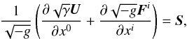 (1)where
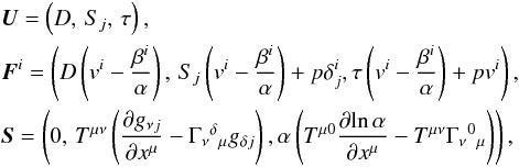 (2)with g = det(gμν) being the four-metric, γ = det(γij) being the three-metric, and
  being the related Christoffel symbols. D is the relativistic density, vi is the three-velocity, Si is the three-momentum, p is the pressure, and τ = E − D is the total energy minus the energy due to the mass. Here, α is the lapse function and βi is the shift vector as defined by the 3 + 1 splitting approach, and W is the Lorentz factor. The energy-momentum tensor Tμν depends on the fluid-type, and we define it for two fluid types in later sections. Full details of the GRHD equations can be found in the work of Banyuls et al. (1997).
We note that the source-terms on the right-hand side of Eq. (2)can also be written as (see documentation for the Whisky code as presented by Baiotti et al. 2003) 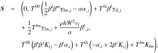 (3)where
 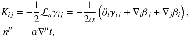 (4)and h is the fluid enthalpy. Equation (3)assumes that the metric is an exact solution of Einstein’s equations. This definition of the sources is equivalent to that in Eq. (2), but is an improvement for numerical solutions as it only uses variables already defined, rather than having to calculate the time derivatives of γij and other space-time variables to incorporate into the 4-Christoffel symbols. In the case of a stationary metric, these are exactly equivalent, but if we had a time-dependent metric (either analytic or numerical), then we would have to find the time derivatives, requiring extra expense and perhaps the use of a finite difference approximation, the accuracy of which would then have to be assessed.
The wavespeeds for the full GRHD system of equations are given by Font (2008, Sect. 6.2): 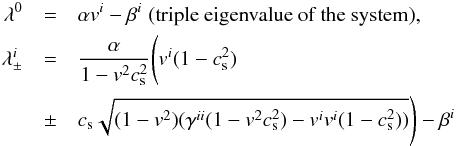 (5)in each coordinate direction i, where there is no sum over the i index. Given an equation of state through the specific enthalpy h, the energy momentum tensor for a perfect fluid is given by
 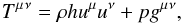 (6)where the four-velocity uμ is defined in terms of the three-velocity vi via
 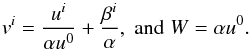 (7)In this paper, we restrict ourselves to two fluid types: a perfect ideal gas, with a given adiabatic index, Γ, and a stiff, ultra-relativistic fluid. We define these in the following sections.
2.1. Stiff fluid
The stiff fluid is a special case of an ultra-relativistic fluid, where, instead of taking p = (Γ − 1)ρ as for an ultra-relativistic fluid, we now take p = ρ. This results in the sound-speed in the fluid being equal to the speed of light, i.e. cs = 1, but does not introduce any further complications.
The fluid is defined in terms of a stream-function ψ, which allows for some simplifications to the fluid equations, resulting in the possibility of analytical solutions (e.g. Petrich et al. 1988; Shapiro 1989). The details of the more general ultra-relativistic fluid can be found in the thesis of Neilsen (1999).
We define the fluid variables as follows:
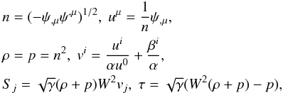 (8)where, due to the inherent simplifications, we can ignore the equation for D. This explains the absence of a −D term in the expression for τ.
The primitive variables are easily recovered from the conserved variables via the formulae  (9)We note that Neilsen (1999) warns against calculating vi in this way due to potential numerical precision problems, but the solution he gives is for one dimension only, and is not easily generalisable to multi-dimensions.
The above equation of state allows the simplification of the equation for conservation of energy and momentum,  , to the linear wave equation
  (although we note that not all solutions of the linear wave equation result in physically valid stiff-fluid solutions).
2.2. Ideal fluid
For the ideal fluid, we define the specific enthalpy of the fluid to be  (10)where Γ is the adiabatic index of the fluid (often written as γ, but that has already been used for the determinant of the three-metric). The speed of sound in the fluid, cs, is then given by
  (11)In non-relativistic fluid evolution, the recovery of the primitive variables from the conserved variables is an algebraic operation. However, the presence of the Lorentz factor complicates the issue, since the three-momenta are no longer independent of each other, and we use a Newton-Raphson method to recover the primitive variables. Other techniques are available, including the solution of a quartic, but tend to be computationally involved and expensive.
For the primitive variable recovery, we follow the approach in Appendix A of Eulderink & Mellema (1995). In order to retain numerical accuracy, we rewrote the expression for calculating u0 = W/α in Eq. (A.12) of Eulderink & Mellema (1995) as  (12)taking C0ξ outside the brackets, since for large W the bracketed expression is of order unity and C0ξ is large.
Although our numerical scheme is designed not to induce unphysical data, this is only proven to be true for scalar conservation laws. In case we encounter unphysical data, we enforce a minimum fluid density. We use the following to recover the remaining primitive variables:  (13)where ρmin = 10-8 (assuming that the equations have been non-dimensionalised with c = 1). Given that ρ may have been altered from its correct value of D/W, we recalculate the appropriate value of p from h, enforce p ≥ pmin if necessary, and then recalculate h before calculating vi as
  (14)Following the preceding scheme, we have not had any problems with unphysical values of variables being generated. We are therefore confident that we have a robust approach to recovering primitive variables.
3. Black hole metrics
In this section we give an overview of the space-time metrics we have used in our simulations. Note that we have expressed these in Cartesian coordinates throughout. Our reasons for doing so are that we wish to have a global coordinate system across all overlapping grids (see Sect. 4.4) and that the coordinate system not have any singularities.
The two main metrics that we consider are:
-
Kerr-Schild: this metric represents a single black-hole with massM, spin a, but no charge. Details are given in Sect. A.1.
-
Boyer-Lindquist: this metric represents the same space-time as Kerr-Schild and has been used in previous work in this area. We do not actively use it in our simulations but refer to it for comparative purposes. Details are given in Sect. A.2.
In order to compare with previous work, we shall need to transform between the Kerr-Schild and Boyer-Lindquist coordinate systems. Details of this transformation are given in Sect. A.3.
As a demonstration of the applications to which our numerical scheme could be put, we also use a binary black-hole system. Here we use Brill-Lindquist initial-data which, when evolved would give rise to an inspiralling binary black-hole system. However, we are not evolving the metric and will only use this for demonstration purposes. Details of the metric are given in Sect. A.4.
4. Numerical schemes
In this section, we describe the numerical scheme we have developed and our adaptation of the scheme to curved space-time. Further details can be found in our previous paper on evolving special relativistic hydrodynamical (SRHD) problems (Blakely et al. 2015).
To summarise the scheme, we use the Slope-LImited Centred (SLIC) scheme described in Toro (1999), based on the GFORCE approximate Riemann solver of Toro & Titarev (2006). As demonstrated in Blakely et al. (2015) this allows us to improve the accuracy of the scheme without needing to derive characteristic information for the system. This modified SLIC scheme is implemented for a curvilinear coordinate system, which entails some extra work to maintain conservation.
The governing equations presented in Eq. (1)can be written in the form of a conservation law:  (15)where u is a general state vector, whose evolution in time is governed by fluxes fj in each dimension and source terms s.
Neglecting the source term, the numerical update formula for this is:  (16)where spatial cells are indexed with i, and time-steps are indexed with n. The fluxes appearing in Eq. (16)are computed using the approach described in the following sections. The time-step Δt is computed as
  (17)where CCFL is the CFL number, Δx is the grid spacing, and Smax is the maximum wave-speed across all cells.
4.1. GFORCE flux
We can express the generalised First-ORdered CEntred (FORCE) flux (GFORCE) of Toro & Titarev (2006) as a weighted average of the Lax-Friedrichs and Lax-Wendroff fluxes, with the weighting depending on local wave speed information. For the case of linear-advection, GFORCE is identical to the Godunov upwind scheme. This suggests that the GFORCE flux could well provide improved accuracy for complex systems of equations compared to the FORCE flux, which does not depend on local wave-speed information. The wave speed calculation is carried out in the local computational grid coordinates so that the wave speeds are aligned with the grid, and the wave-speeds we use for GRHD are those given in Eq. (5).
4.2. Slope limiting
The GFORCE scheme is only first-order accurate. In order to increase the order of accuracy, we use a slope-limited reconstruction of the solution to determine left and right biased solution states at cell-faces for which we can solve a Riemann problem using GFORCE. Full details are given in Blakely et al. (2015). As in the previous paper, we use the van Leer slope-limiter, which we have found to give good shock-capturing properties introducing minimal non-physical oscillations into the solution.
To implement the SLIC scheme we first reconstruct the slope of the solution, Δi, using data from either side of the current cell, taking the average of the forward and backward differences:  (18)and then determine a limited slope
  by multiplying each component by a factor dependent on the local solution behaviour:
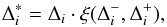 (19)where the limiting function ξ is taken to be
 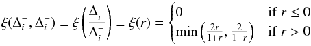 (20)being the van Leer limiter. The preceding two equations are applied to each individual component of Δi,
  , and
, and  to form the limited slope .
The SLIC flux is then calculated according to 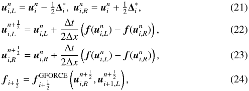 where we use
  and
and  as the left and right states for the GFORCE flux.
4.3. Source terms and operator splitting
In Eq. (2)we see that there are source terms which arise from the non-flat metric. We evolve these separately using a second-order-accurate Runge-Kutta scheme, to match our second-order finite-volume scheme. However, in order to retain second-order accurate evolution overall, when combined with the evolution of the flux terms, we need to use the Strang splitting 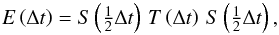 (25)where S is the evolution operator of the source terms, T is the evolution operator of the hyperbolic part of the system, and E is the full evolution operator. As a result E is second order in time if both T and S are.
4.4. Curvilinear overlapping grids
Details of how we adapt the standard finite-volume schemes to work on curvilinear grids are given in Blakely et al. (2015). We give a brief overview of our approach here, in preparation for its extension to a non-flat metric.
We denote the spatial Cartesian coordinates as xi and the coordinate system of the grid as ri, and write the standard conservation law in the following way: 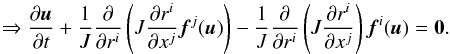 (26)where J is the Jacobian of the coordinate transformation:
 ![Mathematical equation: \begin{equation} J = \left|\left[\frac{\partial x^i}{\partial r^j}\right] \right|\cdot \label{eqn:Jacobian} \end{equation}](/articles/aa/full_html/2015/03/aa25184-14/aa25184-14-eq85.png) (27)The slope-limiting approach is then re-written from Eq. (24)as:
(27)The slope-limiting approach is then re-written from Eq. (24)as:
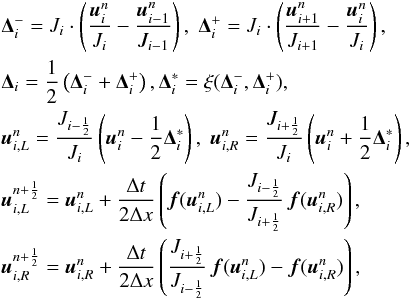 (28)where Ji is the Jacobian of cell i, and we interpolate
  . The derivatives ∂rl/∂xm, however, are averaged using the harmonic mean
 ![Mathematical equation: \begin{equation} \left.\left[\frac{\partial r^l}{\partial x^m}\right]\right|_{x=x_{i+1/2}} = B_{i+\tfrac{1}{2}} = 2\left(B_i^{-1} + B_{i+1}^{-1}\right)^{-1} , \end{equation}](/articles/aa/full_html/2015/03/aa25184-14/aa25184-14-eq90.png) (29)where Bi is the matrix given by
(29)where Bi is the matrix given by ![Mathematical equation: \begin{equation} B_i = \left.\left[\frac{\partial r^l}{\partial x^m}\right]\right|_{x=x_i} . \end{equation}](/articles/aa/full_html/2015/03/aa25184-14/aa25184-14-eq92.png) (30)
(30)
4.5. Evolution on a curved metric
So far we have not made any mention of how we deal with a non-flat metric. Since our intention is to develop numerical schemes that will be of use when the metric is being evolved as well as the fluid, we make the assumption that we only know the metric at the cell centres (i.e. at the same points as the fluid), rather than using analytic values wherever they are needed. However, since the SLIC scheme requires metric values at cell faces, we need to describe how to determine these from cell-centred values. A careful and rigorous approach to this is presented in Rossmanith et al. (2004). However, as this approach is somewhat involved, and computationally expensive, we instead use the following approach, which also includes considerations for a curvilinear coordinate system. This is a generalisation of the SLIC method on flat space, given in Eq. (28), and explicitly uses slope-limiting on primitive variables, rather than conserved variables. In the following we use p for the primitive fluid variables, u for the conserved fluid variables, and g for the metric variables. We also use u(gi,pi) to define the conserved variables u as a function of the primitive variables p and the metric g, where the subscript i refers to the cell in which the quantities are calculated. In the case where the metric is stationary, and is not being evolved, we define
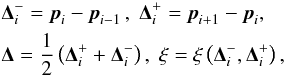 (31)then find slope-limited values
 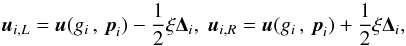 (32)average the metric for cell-faces
  (33)adjust the fluid variables for the cell-face metric
  (34)and then continue as in Eq. (28), replacing
  by the
  found above. These calculations are somewhat expensive since they involve several conversions between primitive and conserved variables. However, we have found them to improve accuracy substantially, particularly for three-dimensional simulations.
The main improvement to the fluid evolution comes through the use of averaging the metric correctly for the cell faces as above. Our reason for using the primitive variables on which to limit is due to the fact that, on a curvilinear grid, the mixing that occurs between different components of the momentum can cause a flow in the x-direction to develop non-zero velocities in the y-direction. Removing the mixing effect of the Lorentz factor on the momenta by limiting on primitive variables reduces this effect, but does not remove it altogether.
4.6. Boundary conditions
In dealing with excised black holes, there are two types of boundary condition that must be considered: inner (excision) boundary conditions, and outer (spatial infinity) boundary conditions.
4.6.1. Excision boundary conditions
At the analytic level, boundary conditions are not needed at an excision boundary, provided that it is within the black hole’s apparent horizon, since no physical information can emerge from an apparent horizon. However, most numerical methods do require numerical boundary conditions as a method may use cells further inside the black hole in order to provide a local reconstruction of the solution. There are methods which overcome this, for example, causal differencing as described by Gundlach & Walker (1999), but they tend to be computationally expensive. Simpler methods can lead to satisfactory solutions if sufficient care is taken with the boundary conditions.
When evolving the fluid, the approach we used was to copy the conserved variables from just inside the grid onto the two ghost cells, multiplying by the ratio of the metric determinants in the respective cells. Any higher-order extrapolation, unless checked carefully with extra routines, could lead to negative densities or pressures, which would immediately cause the method to fail.
4.6.2. Boundary conditions at spatial infinity
We should like to have our outer boundaries at spatial infinity. However, due to limited computational resources, we choose to restrict ourselves to a finite domain. There do exist ways of capturing infinite space-times on a finite grid, such as the use of a conformal mapping of the metric as descibed by Alcubierre et al. (2000) but these require more computational expense and more complex numerical algorithms.
The incoming fluid is defined using fixed Dirichlet boundary conditions, and the boundary conditions where the fluid is outgoing are that the fluid is extrapolated to zeroth-order in conserved variables, where no allowance is made for the change in metric as at the excision boundary, since we assume the metric to be nearly flat there.
4.7. Overlapping grids
There are two main issues with regard to dealing with overlapping grids. The first is that of constructing the full grid structure. This is one of the tasks that Overture1 has been designed to perform for even very complicated grids. Given a set of logically rectangular grids, along with mappings to the physical grid coordinates, as well as boundary conditions, Overture can remove parts of grids that are obscured by other grids and calculate which cells on which grids should be used to interpolate data onto grid cells that are now near cut-out portions of the grid. Cells that are obscured by other grids are masked out, and it is possible within a code, to avoid performing any computations at these points.
We use explicit fifth-order interpolation between grids. With explicit interpolation, the interpolation points only need to use values from the interior of other grids. Each point can therefore be determined as an explicit function of a set of values on the donor grid. Overture performs its interpolation using Lagrange polynomials, and takes into account the grid geometries involved. A possible drawback of using higher-order interpolation is that it is not guaranteed that the interpolated values will be contained in the same range as the values from which they are interpolated. This could lead to overshoots developing at grid boundaries. However, we have not found this to be a problem.
5. Bondi-Hoyle-Lyttleton accretion
Although we have analytic solutions of Einstein’s equations such as the Kerr black hole, black holes will never exist in complete isolation in the physical universe. It is more likely that they will either be close to one or more stars or that they will be moving through an interstellar gas, the latter being known as Bondi-Hoyle-Lyttleton (BHL) accretion. BHL accretion usually refers to the supersonic flow of a gas onto a gravitating accretor, but we specialise to a black hole for our purposes.
The starting assumptions for BHL accretion are that a stationary (fixed centre) black hole is subject to a wind composed of a fluid coming from infinity at Mach ℳ∞ = v∞/c∞, where c∞ is the sound speed in the fluid and v∞ is the fluid speed, both measured at a large distance upstream of the black hole. The black hole has mass M and spin a, and the spin axis may be at any angle to the wind direction. The gas may be of any composition, but we restrict ourselves to the cases of an ideal gas, with adiabatic index Γ, and a stiff fluid. We assume that the accretion of the fluid onto the black hole does not change its mass significantly, i.e. we are using the test-fluid approximation.
5.1. Relativistic BHL accretion
Some axisymmetric simulations of accretion onto a moving black hole were performed by Petrich et al. (1989) using finite-difference methods with artificial viscosity. Following them, there is a series of papers on numerical calculations of accretion rates by Font & Ibáñez (1998a,b) and Font et al. (1999). The most general case studied was that of wind accretion onto a spinning Kerr black hole, using a range of Mach numbers, adiabatic indices, and spin rates. However, these were done either assuming axisymmetry or in the equatorial plane (thin disk approximation), although as described by Font et al. (1999) this latter “dimensional simplification still captures the most demanding aspect of the Kerr background, which is encoded in the large azimuthal shift vector near the horizon”. The reason for these simplifications was limited computational resources, which at the time would not allow high-resolution three-dimensional calculations to be performed in a reasonable time.
Further, the first two of these papers mentioned in the previous paragraph did not use excision, as such. Rather they used Boyer-Lindquist coordinates as described in Appendix A.2, which have a coordinate singularity at the horizon. Font et al. (1999) made use of a tortoise coordinate r∗ in the radial direction such that  (35)for a black-hole of mass M and spin a, so that on the computational grid, the outer event horizon is situated at r∗ = −∞. This defines a grid that becomes ever more refined as it approaches the horizon, without ever reaching it. Any adverse effects caused by not performing the excision within the horizon are thus put at a sufficiently large distance (in computational space) that their effect on the numerical solution are minimised. The third paper in the series by Font et al. (1999), however, did use Kerr-Schild coordinates, and so used excision inside the horizon, although since the setup was two-dimensional only, this was easily achieved by using plane-polar coordinates and enforcing suitable outgoing boundary conditions at some non-zero radius.
5.2. Perturbed Newtonian BHL accretion
Another body of work on BHL accretion is due to Ruffert (1994, 1995, 1997, 1999). These look at Newtonian BHL accretion onto an absorbing compact object. This is similar in nature to the situation in which we have a black hole, but we expect that relativistic effects will affect the results, possibly giving a stabilising effect. Ruffert’s simulations were done in three dimensions for a range of accretor sizes and incident wind directions, using a nest of Cartesian grids at various resolutions (fixed mesh refinement). Ruffert used a fluid whose density was not uniform upstream of the black hole, but which had a non-constant profile perpendicular to the wind direction.
6. Numerical parameters
In this section we detail the specific numerical schemes that we use, and also the grid structure that we use for the problems described above.
6.1. Evolution methods
As outlined in Sect. 4, and from a desire to use as little computing power as possible, we have decided to use the GFORCE scheme for flux evaluation, using piecewise-linear reconstruction, with the van Leer slope-limiter limiting on primitive variables. We use the RK2 scheme for evaluating source terms, and a CFL parameter of 0.95.
6.2. Grid setup
There are several possibilities for creating a spherical grid with no polar singularities. The most well-known are the Yin-Yang grid as described by Kageyama (2005), where two identical grids mesh to form the entire sphere, and the cubed sphere, where six identical patches are used to cover the sphere, arranged like the sides of a cube. The latter is the approach used by Zink et al. (2008) and adapted to cover the interior of the spherical domain if necessary by the inclusion of a central seventh grid.
However, for our simulations, we have used the following scheme to remove the polar singularity:
-
Take two identical hollow spheres.
-
Remove their polar singularities by restricting the latitudinal coordinate to θ ∈ [θmin,θmax] = [0.18π,0.82π].
-
Rotate one sphere through π/ 2 about a line perpendicular to its axis.
-
Combine the two spheres to form an overlapping grid.
The resulting grid is shown in Fig. 1.
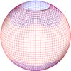 |
Fig. 1 Overlapping grid structure used for three-dimensional simulations. It is formed from two hollow spheres. The blue sphere is not wholly present as parts of it have been removed where it covers the same regions as the red sphere. |
We have defined our grid so that the grid cells are always approximately cubic. To this end, we have used a stretching transformation that makes the grid spacing in the radial direction proportional to the radius. Further, the numbers of cells in the φ (longitudinal) and θ (latitudinal) directions are determined so that the cells are approximately cubic. The numbers of cells in the φ and θ directions are defined as
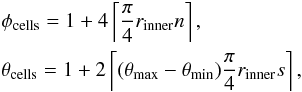 (36)where s is a number characterising the resolution of the grid, rinner is the excision radius, and router is the outer radius. The number of radial cells is then defined as
 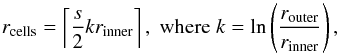 (37)and the transformation of the radial coordinate is defined as
 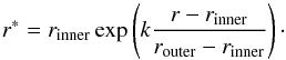 (38)This is a transformation from [rinner,router] to itself, and clearly
  as required to maintain approximately cubic cells.
Although the resolution parameter n does not have a trivial relationship with the number of cells in the grid, the setup remains such that doubling s will multiply by eight the number of cells in the grid overall. The relation with the minimum grid-cell size is not as trivial, however, due to the non-linear mapping from computational space onto physical space.
Although the outer horizon of a spinning black hole is not spherical, we always use a spherical excision boundary. The ellipsoidal outer horizon has a circular cross-section in the equatorial plane, with (Cartesian) radius  (39)and the minor axis of the horizon lies on the z-axis, and corresponds to a radius
  (40)where we have taken the black-hole mass to be M = 1, leaving it characterised only by its spin a.
We therefore ensure that our spherical excision boundary is within the latter radius, so that the whole of the region (up to a large spatial distance) outside the outer horizon is covered by the computational grid. The excision radii for the three spins we use are given in Table 1. The scheme used to calculate them also ensures that the two ghost cells inside the excision boundary still lie outside the inner horizon.
Set of radii at which we perform spherical excision, ensuring that the excision is inside the outer horizon.
Grid cell statistics for the resolutions used.
The parameters of the grids we have used for our results are shown in Table 2. There are three resolutions, which we will refer to as low, medium, or high, corresponding to s = 35, 50, 60 respectively.
6.3. Mass and momentum accretion
In order to calculate the mass accretion rate Ṁ from our numerical output, we note that, following Petrich et al. (1989):
![Mathematical equation: \begin{eqnarray} && \partial_\mu(\sqrt{-g}J^\mu) = \sqrt{-g}\nabla_\mu J^\mu = 0, \nonumber \\[1mm] && \text{where}\;J^\mu=\rho u^\mu\;\text{is the conserved four current,}\\[1mm] && \text{and}\;\sqrt{-g}=\alpha\sqrt{\gamma}, \nonumber \end{eqnarray}](/articles/aa/full_html/2015/03/aa25184-14/aa25184-14-eq141.png) (41)where g is the four-metric, γ the three-metric, and α the lapse function.
(41)where g is the four-metric, γ the three-metric, and α the lapse function. ![Mathematical equation: \begin{eqnarray} \text{Then},\;\text{since}\; u^0&=&W/\alpha, \nonumber \\[2mm] M&=&\int_V\sqrt{\gamma}\rho W \mathrm{d}V = \int_V\sqrt{-g}J^0 \mathrm{d}V ,\nonumber \\[2mm] \hspace*{-1cm}\text{so that}\hspace*{0.85cm}\dot M&=&\int_V\frac{\partial}{\partial x^0}\left(\sqrt{\gamma}D\right)\,\mathrm{d}V = \int_V\frac{\partial}{\partial x^0}\left(\sqrt{-g}J^0\right)\,\mathrm{d}V\nonumber \\[2mm] &=&\int_V\sqrt{-g}{0}{\nabla_\mu J^\mu} - \partial_i\left(\sqrt{-g}J^i\right)\,\mathrm{d}V\nonumber \\[2mm] &=&-\int_S\sqrt{-g}\rho u^i\,\mathrm{d}\vec{S}_i\nonumber \\[2mm] &=&-\int_S\alpha\sqrt{\gamma}\rho W\left(v^i - \frac{\beta^i}{\alpha}\right)\,\mathrm{d}\vec{S}_i. \end{eqnarray}](/articles/aa/full_html/2015/03/aa25184-14/aa25184-14-eq142.png) (42)In order to evaluate Ṁ numerically, we interpolate the integrand at evenly spaced points in the θ and φ coordinates around a sphere with some radius r. These are then summed, weighted by the areas ΔSi = γijnjΔA at those points. We use 150 points in the θ (latitudinal) direction and 300 points in the φ (longitudinal) direction. This is a sufficient number of points as we show in Sect. 7.2.
(42)In order to evaluate Ṁ numerically, we interpolate the integrand at evenly spaced points in the θ and φ coordinates around a sphere with some radius r. These are then summed, weighted by the areas ΔSi = γijnjΔA at those points. We use 150 points in the θ (latitudinal) direction and 300 points in the φ (longitudinal) direction. This is a sufficient number of points as we show in Sect. 7.2.
We compute the integral in Kerr-Schild coordinates, which differs from Font & Ibáñez, who calculated the integral in Boyer-Lindquist coordinates. However, as the result is a scalar, it should be the same in both coordinate systems.
In Petrich et al. (1988), however, the density ρ in the above is replaced by  , the baryon density, and so for comparisons with their exact solution, we use this slightly altered expression when dealing with a stiff fluid.
7. Validation of code
Although in Blakely et al. (2015) we presented validation of our code for a flat metric in simple 1D cases, and also in 2D cases, we have not yet shown that our algorithm is robust enough to evolve three-dimensional flows for very long periods of time accurately. Further, there may be boundary condition issues, both at the excision boundary and at the outer boundary that need to be rectified. We therefore seek to test our code against known results for BHL accretion.
7.1. Exact solutions
There is a surprisingly general exact solution for wind accretion, derived by Petrich et al. (1988). Here, an exact, stationary solution for the accretion of a stiff fluid (see Sect. 2.1) onto a Kerr black hole in Boyer-Lindquist coordinates is presented. The solution is given for a black hole of mass M, any spin a, and for any direction of incidence of the wind, by the components of the four-velocity uμ and the density n as follows: ![Mathematical equation: \begin{eqnarray} n\cdot u_t\, &=&-u_\infty^0, \nonumber \\ n\cdot u_r &=& -\left(r_+^2+a^2\right)\frac{u_\infty^0}{\Delta} + u_\infty\cos{\theta}\cos{\theta_0} \nonumber \\ && +~u_\infty\Re\left(\left[1 + \mathrm{i}a(r-M+\mathrm{i}a)/\Delta\right] \times \sin{\theta}\sin{\theta_0}\,\mathrm{e}^{\mathrm{i}(\phi - \phi_0 - \chi)}\right), \nonumber \\ \label{eqn:Wind_exact} n\cdot u_\theta &=& -u_\theta(r-M)\sin{\theta}\cos{\theta_0} \\ && +~u_\infty\Re\left[\left(r-M+\mathrm{i}a\right)\cos{\theta} \sin{\theta_0}\, \mathrm{e}^{\mathrm{i}(\phi-\phi_0-\chi)} \right], \nonumber \\ n\cdot u_\phi &=& -u_\infty\Im\left[\left(r-M+\mathrm{i}a \right)\sin{\theta}\sin{\theta_0}\,\mathrm{e}^{\mathrm{i}(\phi-\phi_0-\chi)}\right],\nonumber\\ n^2 \,\,=&& \hspace*{-3mm} \left[\left(r^2+a^2\right)u_\infty^0 - a\cdot \left(n\cdot u_\phi\right)\right]^2/(\Sigma\Delta)\nonumber\\ &&\hspace*{-3mm} -~ \left[\left(nu_\phi\right) - a\sin^2{\theta}\left(u_\infty^0\right)\right]^2/\left(\Sigma\sin^2{\theta}\right)\nonumber\\ &&\hspace*{-3mm} -~ \left(\Delta/\Sigma)(nu_r\right)^2 - \left(nu_\theta\right)^2/\Sigma,\nonumber \end{eqnarray}](/articles/aa/full_html/2015/03/aa25184-14/aa25184-14-eq146.png) (43)where
(43)where  (44)The incident direction angles θ0 and φ0 are extracted from the vector vi, being the polar angles corresponding to the wind direction, and Δ is defined in Eq. (A.6).
The mass accretion rate is then found to be  (45)and the stagnation point of the fluid is at
 ![Mathematical equation: \begin{equation} r=M\left[1 + \sqrt{1+\frac{4}{v_\infty}} \right], \end{equation}](/articles/aa/full_html/2015/03/aa25184-14/aa25184-14-eq153.png) (46)for the case of zero spin.
(46)for the case of zero spin.
This solution is not in the correct form for our purposes, however, as it uses Boyer-Lindquist coordinates which are singular at the horizon. We therefore use the coordinate transformation given by Eq. (A.10)to transform the velocity to the Kerr-Schild coordinate system.
7.2. Validation results
We now present the results of applying our code to the exact solution for wind accretion of Petrich et al. presented above. When taking cross sections of the solutions, we do so along the x-axis, since we have the wind coming in from x = −∞ by default. We do not plot raw values of the solution at grid points, but interpolate 800 equally spaced points between x = ± 50M. Therefore, our plots show the correct shape of our evolved solution, but not raw numerical values. We note that for the low resolution grid (see Table 2), 100M/ Δrmin ≈ 1700, so 800 points is certainly not too many to use for the interpolation, at least near the horizon.
Evolving the solution of Petrich et al. will test all parts of our code, as it requires the capturing of effects that do not have spherical or Cartesian symmetry, so that all flux components are tested, along with our implementation of evolution on curvilinear grids. The suitability of both the inner and outer boundary conditions will also be tested.
Unless otherwise stated, the following tests are all carried out using a low resolution grid (see Table 2) with an inner boundary at r = M and an outer boundary at r = 50M. We use a fluid velocity at infinity of v∞ = 0.6, so as to compare to Fig. 1 in Petrich et al. We perform an evolution starting with a constant density and constant velocity field, adjusted near the black-hole to avoid unphysical states. (This is the same initial conditions as we use for later simulations.)
A comparison of the exact and numerical solutions is shown in Fig. 2. The differences between the exact solution and the numerical solution is shown in Fig. 3. We see that although the solutions appear fairly close except near the outer boundaries, the relative difference between the exact and numerical solutions is somewhat larger than that from evolving the exact solution as initial data. We note that there are interesting effects at the boundaries, and we believe these to be due to boundary conditions not necessarily being sufficiently accurate for subsonic flow. However, we believe that our results are sufficiently accurate as mass accretion rates are reasonably accurate for the relatively low resolution that we use.
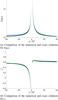 |
Fig. 2 Comparison of the numerical and exact solutions for log ρ and vx. The numerical solution is given by the blue plus-signs and the exact solution is given by the green triangles. |
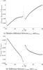 |
Fig. 3 A stiff fluid with an initial state of ρ = 1 and |

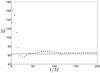 |
Fig. 4 Mass accretion rate Ṁ resulting from evolving constant intial conditions to time t = 200M, evaluated at radius r = 5M. The solid line shows the exact solution, and the plus-signs the numerical solution. |
The mass accretion rate Ṁ, shown in Fig. 4, stabilises to a constant limit after a time of about 130M. The limit is slightly in excess of the analytic value, exceeding it by about 4.3%. We note that increasing the outer radius of the domain did not seem to correct this.
Convergence of the accretion-rate with increasing resolution parameter s.
We performed a simple convergence study, evaluating the mass accretion rate at radius r = 5M, after time T = 200M, for three resolutions, shown in Table 3. If we assume a convergence relation of the form ϵ = ks− p, then this yields  . This suggests that we are slowly converging to the exact solution. We believe that the slow convergence is connected to incorrect subsonic boundary conditions at a finite radius. Applying our code to a stiff fluid accretion onto a BH with spin a = 0.5 results in the mass accretion rate evolving as shown in Fig. 5. We see that the limiting value resulting from the evolved solution is slightly in excess of the analytic solution, this time by about 4.1%.
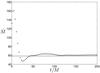 |
Fig. 5 Variation in time of the mass accretion rate of a stiff fluid with velocity v∞ = 0.6 onto a Kerr black hole with spin a = 0.5. The analytic solution as derived by Petrich et al. is shown by the line, and the numerical solution is shown by the +s. |
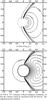 |
Fig. 6 Steady-state fluid for model UB1 with uniform flow and a non-spinning black hole at time t = 400M. The medium resolution grid was used, and the axes are scaled in terms of the accretion radius ra = 0.92M. |
7.3. Comments on validation
We have demonstrated that our code is capable of reproducing the exact solution of Petrich et al. to a good accuracy. The fact that the solution converges to a steady state shows that the appropriate quantities are conserved. It is clear that our outer boundary conditions, although only defined at a finite radius, are sufficiently far away not to affect the solution adversely. We note, however, that there are some issues with the solution near the inflow boundary conditions. We suspect that these are related to our implementation of the outer boundary conditions for subsonic flow, and this may be the cause of the poor convergence rate illustrated above. This would require further effort to handle correctly and consistently. Further, the results have been obtained at a relatively low resolution, which points to the overall accuracy of our method.
Therefore, we conclude that our numerical methods are robust and accurate, and that the results and conclusions we present in the next section are therefore valid.
8. Validation against previous work
In order to validate our code for use in modelling Bondi-Hoyle-Lyttleton accretion, we use one of the models suggested by Font & Ibáñez (1998b). Specifically, we use their model UB1, which has the parameters:  (47)For a more direct comparison with Font & Ibáñez (1998b), we have scaled the mass accretion rate in the same way, by a factor
  In Fig. 6 we show the results for running the UB1 model to time t = 400M on a medium resolution grid (see Table 2). We have plotted the same contour levels and used the same figure limits as Font & Ibáñez (1998b). We evolve to steady state, as do they, although we show our results at a later time. For the velocity plot, we have transformed into Boyer-Lindquist coordinates for a direct comparison. The plot of density shows somewhat higher densities than those of Font & Ibáñez. The velocity plot shows the stagnation point at r = 5.65M as being slightly further downstream than that found by Font & Ibáñez at r = 5.22M, but the contours are otherwise visually very similar.
In Fig. 7 we plot the mass accretion rate as a function of time. As expected, it tends to a constant limit since we have reached a steady state. Evaluating the mass accretion rate at a smaller radius does not affect the limiting value, either, again showing that the flow is at a steady state. However, the final rate of Ṁ = 34.3 is somewhat higher than the final (scaled) mass accretion rate found in Font & Ibáñez (1998b), which suggested it to be Ṁ = 27.0. The difference in the evolution of the mass accretion rates (ours shows a peak at time t ≈ 10M, while Font & Ibáñez (1998b) show a monotonic increase to the final limit) is explained by the difference in coordinate systems, and hence initial conditions, as we specified initial velocity to be constant in Kerr-Schild coordinates, as opposed to Font & Ibáñez’s use of Boyer-Lindquist coordinates. The difference in the final mass accretion rate may be due to either their slightly lower resolution, or a difference in the far-field boundary conditions.
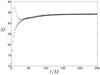 |
Fig. 7 Mass accretion rate for the UB1 model evaluated at r = 2.5M (circles) and r = 5M (+ signs). |
8.1. Testing spherical symmetry
Although our physical domain is spherical, the grids do not have spherical symmetry, due to the overlapping grid structure (see Fig. 1). In Table 4, we show the effect of θw, the incident angle of the inflowing fluid, on the mass accretion rate for a non-spinning black-hole when using the low resolution grid. In theory, of course, there should be no difference due to the symmetry of the configuration. We do, however, see a small difference in the accretion rates. The fact that the results for θw = 0,π/ 2 and θw = π/ 6,π/ 3 are very similar, with differences at most 0.3%, suggests that the errors are either linked to the angle with a Cartesian axis, or with the interpolation boundary at θw = π/ 4.
The effects we have noticed here, though, are relatively small. We therefore conclude that we can safely use the low resolution grid to obtain good results in as little computational time as possible.
Effect of θw on mass accretion rate for non-spinning black hole, at time t = 300M, evaluated at radius r = 5M.
9. Perturbed accretion onto a spinning BH
We have performed a comprehensive analysis of how spin and density perturbations affect the accretion. However, for reasons of space, we shall publish this full investigation separately, and here give just a single result from our study.
We initialise our simulation with the following density profile upstream (the flow direction is from x = −∞) ![Mathematical equation: \begin{equation} \rho_\infty=\rho_0\left(1-\frac{1}{2}\tanh\left[2\epsilon_\rho\frac{y}{R_{\rm A}}\right]\right),\\ \end{equation}](/articles/aa/full_html/2015/03/aa25184-14/aa25184-14-eq200.png) (50)where the accretion radius is defined to be
(50)where the accretion radius is defined to be  (51)and we set parameters
  (52)and other fluid parameters from the UB1 model. Note that the perturbed density profile is maintained by explicitly setting the boundary conditions at all times.
In Fig. 8 we show the final steady-state density and velocity cross-sections of the accretion problem. The fluid accretes from the left, and the black hole’s horizon is shown as a dashed line, and it is spinning about an axis perpendicular to the page, and in an anti-clockwise direction.
 |
Fig. 8 Contour plots of density and velocity for a supersonic flow with density perturbed by ϵρ = 0.2 past a black hole with spin a = 0.9 and flow parameters given by model UB1. The plots are evaluated at time t = 300M, and the axes are in units of M. |
We see that a shock-cone has formed downstream of the black hole. Due to the effect of the black hole’s spin, the points where the shock-cone attaches to the horizon have been dragged round. This feature was also found by Font & Ibáñez in their study, that the effect of the spin did not extend to spatial infinity, but was restricted to the immediate vicinity of the horizon. However, the effect of the perturbed density is to pull the shock-cone further round in the anti-clockwise direction. The reason that it does so is that the fluid in the upper half of the domain is at a lower density than that in the lower half. Therefore, the fluid from the lower half has a larger momentum, and can therefore penetrate into the upper half of the domain before being slowed sufficiently to fall into the black hole.
We also see, in both the density and velocity plots, evidence of the shock-cone being split into two by a region of lower density. This feature can also be seen in the work on perturbed accretion of Ruffert (1999), again providing strong evidence that our simulations are consistent with previous work.
10. Accretion onto a BBH system
In order to demonstrate the generality of our approach in using overlapping grids, we present an example of accretion onto a binary black-hole system, represented by the Brill-Lindquist coordinate system. We note that we do not yet have the facility to evolve the metric within our code, so that the black holes remain stationary.
Since the time for which we evolve this setup is several times longer than it would take for the BBH system to inspiral and collapse to a single black-hole, we do not claim that these results have any physical relevance. However, they do demonstrate how straightforward it is for our code to deal with multiple black-holes and excise multiple singularities.
10.1. Simulation setup
For our flow parameters, we use adiabatic index Γ = 4/3, Mach number ℳ = 1.5, and asymptotic upstream sound speed c∞ = 0.1. Font & Ibáñez (1998b) show that when accreting onto a single black hole, this flow results in a wide shock-cone which is almost detached from the upwind side of the horizon.
We specify the black holes to have unit mass and to be positioned at (0, ± 5, 0), with the flow coming along the x-axis. We evolve the flow to a time t = 2000M, and note that the time to merger of a pair of equal mass black holes at this separation is somewhat smaller, at around 250M, than the simulation time.
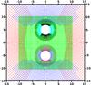 |
Fig. 9 Cross-section of the grid structure used for the binary black hole simulation, in the z = 0 plane. The two black holes are centred at (0, ± 5, 0). Two pairs of spherical grids (black and cyan, and blue and magenta) are used to capture the excision boundaries of the black holes, a Cartesian grid (green) surrounds them, and a third pair of spherical grids (blue and red) is used to capture the outer spatial boundary at 50M. This uses 4 195 765 grid points in total and 500 516 interpolation points. |
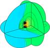 |
Fig. 10 Result of a fluid flowing onto a binary black hole system, with the metric kept stationary. There are two black holes with unit mass at (0, ± 5, 0) in the Brill-Lindquist metric. The fluid upstream of the binary system has adiabatic index Γ = 4/3, Mach number ℳ = 1.5, and asymptotic sound speed c∞ = 0.1. We show the density, with contours evenly spaced between ρ = 0 and ρ = 21. |
We used the symmetric grid setup shown in Fig. 9. Here, we have used two small pairs of grids (the pairs do not overlap each other) to excise the two black holes, covered them with a Cartesian grid, and finally encased the Cartesian grid in a third pair of spherical grids, centred at the origin, and extending out to 50M. Portions of the (green) Cartesian grid have been removed in order to allow the two excision spheres to be captured smoothly. The outer pair of spherical grids extend into the inner black hole grids; this should probably be avoided in general, to avoid interpolation between mismatched grids, but removing this would require the Cartesian grid to be made much larger, resulting in a larger number of grid cells.
The two pairs of grids covering the black holes have inner radii 1.4M and outer radii 4M so that they do not overlap. The Cartesian grid covers the region −10M ≤ x,y,z ≤ 10M, and the outer pair of grids have inner radius 6M and outer radius 50M. This grid setup is symmetric with respect to the two black holes.
10.2. Results
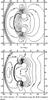 |
Fig. 11 Contour plots for accretion onto a system of two unit-mass black holes at (0, ± 5, 0) using the Brill-Lindquist metric. The fluid state upstream is given by ℳ∞ = 1.5, c∞ = 0.1, ρ∞ = 1, and Γ = 4/3. |
A three-dimensional view of the resulting flow at t = 2000M is shown in Fig. 10. We see that a wide shock-cone has developed, although it is now detached from both of the black hole horizons. There are regions of high density to either side of the gap between the holes, as well as some regions of lower density on the outside edges of the horizons.
Some more quantitative results are shown in Fig. 11. The density plot shows the shock cone forming upstream of the black holes, with density increasing towards them. The density also increases as the black holes are approached from the downstream direction, and the region of highest density is located symmetrically between the black holes, slightly downstream of their centres. The velocity plot also shows the shock-cone, and that the flow decelerates across it. We see regions of low velocity both downstream and upstream of the black holes.
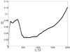 |
Fig. 12 Mass accretion rate for the binary black hole simulation. This was calculated on a sphere radius 10M. |
In Fig. 12 we show the rate at which mass accretes onto the two black holes, evaluated on a sphere of radius r = 10M, i.e. enclosing both black holes. The simulation has clearly not reached a steady state even at t = 2000M.
10.3. Comments
We have shown that our methodology is capable of being applied to a problem where the grid setup is not trivial, and requires the features of Overture to generate the interpolation correctly. If we were to apply our algorithm to the case of inspiralling black holes, we could generate two moving pairs of spherical grids for the two black holes, and then a Cartesian grid that adapted itself to only just contain the two small spherical grids. The outer pair of far-field grids could, however, remain fixed.
11. Conclusions
In this paper, we have extended our previous work for SRHD to GRHD on curvilinear grids. We have given details of how our schemes have to be adapted to deal with a non-flat space-time metric, and presented simulations validating our approach by comparison with an exact solution of wind accretion onto a black hole. We have also compared our code against previous work and shown that our results are qualitatively consistent, although our quantitative results show some discrepancy.
If we were to include evolution of the metric within our code, we would have the added issue that the singularities could move. However, it would be possible to detect apparent horizons to determine their locations. From these, we could dynamically generate spherical grids centred on the singularities, and interpolate the solution between grid systems. Overture has the capability to perform this interpolation for moving grid systems. Alternatively, we could solve the equations in the moving grid frame.
Available from www.OvertureFramework.org
Acknowledgments
This work was funded by an EPSRC Doctoral Training Grant, and use was also made of the Darwin Supercomputer of the University of Cambridge High Performance Computing Service (http://www.hpc.cam.ac.uk/), provided by Dell Inc. using Strategic Research Infrastructure Funding from the Higher Education Funding Council for England.
References
- Alcubierre, M., Brügmann, B., Dramlitsch, T., et al. 2000, Phys. Rev. D, 62, 044034 [NASA ADS] [CrossRef] [MathSciNet] [Google Scholar]
- Baiotti, L., Hawke, I., Montero, P. J., & Rezzolla, L. 2003, Mem. Soc. Astron. It. Suppl., 1, 210 [Google Scholar]
- Banyuls, F., Font, J. A., Ibáñez, J. M., Martí, J. M., & Miralles, J. A. 1997, ApJ, 476, 221 [NASA ADS] [CrossRef] [Google Scholar]
- Blakely, P. M., Nikiforakis, N., & Henshaw, W. D. 2015, A&A, 575, A102 [NASA ADS] [CrossRef] [EDP Sciences] [Google Scholar]
- Boyer, R. H., & Lindquist, R. W. 1967, J. Math. Phys., 8, 265 [NASA ADS] [CrossRef] [Google Scholar]
- Brown, D. L., Chesshire, G. S., Henshaw, W. D., & Quinlan, D. J. 1997, in Proc. Eighth SIAM Conference on Parallel Processing for Scientific Computing [Google Scholar]
- Dönmez, O., Zanotti, O., & Rezzolla, L. 2011, MNRAS, 412, 1659 [NASA ADS] [CrossRef] [Google Scholar]
- Eulderink, F., & Mellema, G. 1995, A&AS, 110, 587 [NASA ADS] [Google Scholar]
- Farris, B., Liu, Y., & Shapiro, S. 2010, Phys. Rev. D, 81, 084008 [NASA ADS] [CrossRef] [Google Scholar]
- Font, J. A. 2008, Liv. Rev. Rel., 11, 7 [Google Scholar]
- Font, J. A., & Ibáñez, J. M. 1998a, MNRAS, 298, 835 [NASA ADS] [CrossRef] [Google Scholar]
- Font, J. A., & Ibáñez, J. M. 1998b, ApJ, 494, 297 [NASA ADS] [CrossRef] [Google Scholar]
- Font, J. A., Ibáñez, J. M., & Papadopoulos, P. 1999, MNRAS, 305, 920 [NASA ADS] [CrossRef] [Google Scholar]
- Gundlach, C., & Walker, P. 1999, Class. Quant. Grav., 16, 991 [NASA ADS] [CrossRef] [Google Scholar]
- Jaranowski, P., & Schäfer, G. 2002, Phys. Rev. D, 65, 127501 [NASA ADS] [CrossRef] [Google Scholar]
- Kageyama, A. 2005, J. Earth Simulator, 3, 20 [Google Scholar]
- Kelly, B. J. 2004, Ph.D. Thesis, College of Science, https://etda.libraries.psu.edu/paper/6289/1562 [Google Scholar]
- Moreno, C., Núñez, D., & Sarbach, O. 2002, Class. Quant. Grav., 19, 6059 [NASA ADS] [CrossRef] [Google Scholar]
- Neilsen, D. W. 1999, Ph.D. Thesis, University of Texas at Austin, http://laplace.physics.ubc.ca/Theses/Phd/neilsen.pdf [Google Scholar]
- Penner, A. J. 2011, MNRAS, 414, 1467 [NASA ADS] [CrossRef] [Google Scholar]
- Petrich, L. I., Shapiro, S. L., & Teukolsky, S. A. 1988, Phys. Rev. Lett., 60, 1781 [NASA ADS] [CrossRef] [Google Scholar]
- Petrich, L. I., Shapiro, S. L., Stark, R. F., & Teukolsky, S. A. 1989, ApJ, 336, 313 [NASA ADS] [CrossRef] [Google Scholar]
- Rossmanith, J. A., Bale, D. S., & LeVeque, R. J. 2004, J. Comput. Phys., 199, 631 [NASA ADS] [CrossRef] [MathSciNet] [Google Scholar]
- Ruffert, M. 1994, ApJ, 427, 342 [NASA ADS] [CrossRef] [Google Scholar]
- Ruffert, M. 1995, A&AS, 113, 133 [NASA ADS] [Google Scholar]
- Ruffert, M. 1997, A&A, 317, 793 [NASA ADS] [Google Scholar]
- Ruffert, M. 1999, A&A, 346, 861 [NASA ADS] [Google Scholar]
- Shapiro, S. L. 1989, Phys. Rev. D, 39, 2839 [NASA ADS] [CrossRef] [Google Scholar]
- Toro, E. 1999, Riemann solvers and numerical methods for fluid dynamics, 2nd edn. (Springer-Verlag) [Google Scholar]
- Toro, E., & Titarev, V. 2006, J. Comput. Phys., 216, 403 [NASA ADS] [CrossRef] [Google Scholar]
- Zink, B., Schnetter, E., & Tiglio, M. 2008, Phys. Rev. D, 77, 103015 [NASA ADS] [CrossRef] [Google Scholar]
Appendix A: Black-hole metrics
In this Appendix we give details of the black-hole metrics we have used in our simulations. These need to be written in a Cartesian coordinate system and, since this is not often given explicitly in GR references, we give full details here for clarity.
Appendix A.1: Kerr-Schild coordinates
The most general black hole we will consider here is the Kerr black hole, with spin, but no charge. The mass of the black hole is M and its dimensionless spin parameter is a where | a | < 1. The metric can be expressed in Cartesian coordinates as follows (Kelly 2004; Moreno et al. 2002):
 (A.1)and this is the form that we use in our code.
There is a more standard form of the metric, in Kerr-Schild spherical coordinates which are defined by Boyer & Lindquist (1967)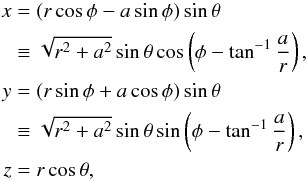 (A.2)where the 3 + 1 split of the metric now takes the form
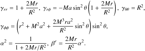 (A.3)The space-time has an outer horizon at r = r+ and an inner horizon at r = r−, where
 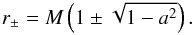 (A.4)
(A.4)
Appendix A.2: Boyer-Lindquist coordinates
Although we use Kerr-Schild coordinates in all of our simulations, we note that previous work in this area has used Boyer-Lindquist coordinates, which we therefore present here as we shall need to use them for comparative purposes.
A black-hole metric can be written in Boyer-Lindquist coordinates, where 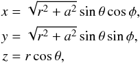 (A.5)which differ from Kerr-Schild spherical coordinates only in the φ coordinate when a ≠ 0. In these coordinates, the metric becomes (again, see Boyer & Lindquist 1967 and Kelly 2004)
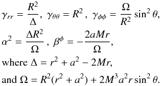 (A.6)This form of the metric has coordinate singularities where Δ = 0, corresponding to the outer and inner horizons. The metric therefore does not extend continuously to inside the event horizon of the black hole, in the same way as the Schwarzschild coordinates, which are a specialization of the Boyer-Lindquist coordinates for a = 0.
Appendix A.3: Transformation between Kerr-Schild and Boyer-Lindquist systems
We shall need to transform velocity vectors between the Kerr-Schild and Boyer-Lindquist coordinate systems. The transformations between Cartesian and spherical coordinate systems are achieved via the transformation tensors 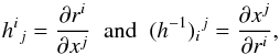 (A.7)where ri are the spherical coordinates (given by Eq. (A.2)or Eq. (A.5)) and xj are the Cartesian coordinates. One-tensors are then transformed from the Cartesian basis to the spherical basis by
  (A.8)and from the spherical basis to the Cartesian basis by
  (A.9)The transformation between Kerr-Schild and Boyer-Lindquist spherical coordinates is then given by Font et al. (1999) as follows:
 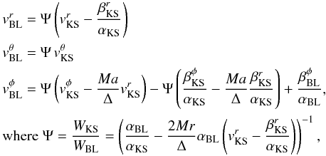 (A.10)where the subscripts KS and BL refer to variables expressed in Kerr-Schild and Boyer-Lindquist spherical coordinates, respectively, and where
  ,
,  are the components of the Eulerian velocity, related to the proper velocity by Eq. (7). Note that Ψ here is the reciprocal of that defined in Font et al. (1999); however, the expressions given here are correct.
Appendix A.4: Binary black holes
In order to demonstrate the generality of our approach to the computational grid structure, we shall demonstrate the evolution of a fluid on a metric containing two singularities. Although we shall not evolve the metric, rendering the simulation physically unrealistic, this will demonstrate the ability of our code to deal with complex grid structures.
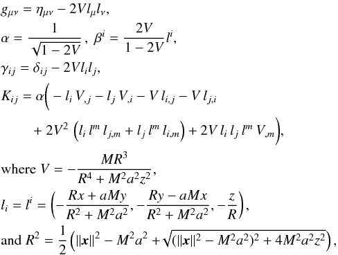
We use Brill-Lindquist initial data, which encapsulates two (non-spinning) black holes with arbitrary masses m1 and m2, at positions x1 and x2. The metric is then given by Jaranowski & Schäfer (2002): 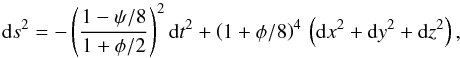 (A.11)where
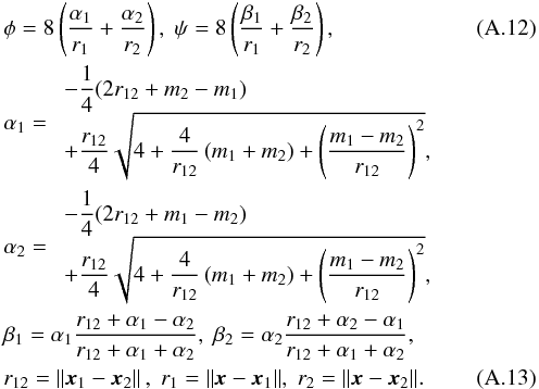 The extrinsic curvature Kij is zero, as is the shift vector βi. This data, when evolved, would rise to a head-on collision of two BHs. However, we reiterate that we do not evolve the metric in our code.
All Tables
Set of radii at which we perform spherical excision, ensuring that the excision is inside the outer horizon.
Effect of θw on mass accretion rate for non-spinning black hole, at time t = 300M, evaluated at radius r = 5M.
All Figures
|
Fig. 1 Overlapping grid structure used for three-dimensional simulations. It is formed from two hollow spheres. The blue sphere is not wholly present as parts of it have been removed where it covers the same regions as the red sphere. |
| In the text | |
|
Fig. 2 Comparison of the numerical and exact solutions for log ρ and vx. The numerical solution is given by the blue plus-signs and the exact solution is given by the green triangles. |
| In the text | |
|
Fig. 3 A stiff fluid with an initial state of ρ = 1 and |
| In the text | |
|
Fig. 4 Mass accretion rate Ṁ resulting from evolving constant intial conditions to time t = 200M, evaluated at radius r = 5M. The solid line shows the exact solution, and the plus-signs the numerical solution. |
| In the text | |
|
Fig. 5 Variation in time of the mass accretion rate of a stiff fluid with velocity v∞ = 0.6 onto a Kerr black hole with spin a = 0.5. The analytic solution as derived by Petrich et al. is shown by the line, and the numerical solution is shown by the +s. |
| In the text | |
|
Fig. 6 Steady-state fluid for model UB1 with uniform flow and a non-spinning black hole at time t = 400M. The medium resolution grid was used, and the axes are scaled in terms of the accretion radius ra = 0.92M. |
| In the text | |
|
Fig. 7 Mass accretion rate for the UB1 model evaluated at r = 2.5M (circles) and r = 5M (+ signs). |
| In the text | |
|
Fig. 8 Contour plots of density and velocity for a supersonic flow with density perturbed by ϵρ = 0.2 past a black hole with spin a = 0.9 and flow parameters given by model UB1. The plots are evaluated at time t = 300M, and the axes are in units of M. |
| In the text | |
|
Fig. 9 Cross-section of the grid structure used for the binary black hole simulation, in the z = 0 plane. The two black holes are centred at (0, ± 5, 0). Two pairs of spherical grids (black and cyan, and blue and magenta) are used to capture the excision boundaries of the black holes, a Cartesian grid (green) surrounds them, and a third pair of spherical grids (blue and red) is used to capture the outer spatial boundary at 50M. This uses 4 195 765 grid points in total and 500 516 interpolation points. |
| In the text | |
|
Fig. 10 Result of a fluid flowing onto a binary black hole system, with the metric kept stationary. There are two black holes with unit mass at (0, ± 5, 0) in the Brill-Lindquist metric. The fluid upstream of the binary system has adiabatic index Γ = 4/3, Mach number ℳ = 1.5, and asymptotic sound speed c∞ = 0.1. We show the density, with contours evenly spaced between ρ = 0 and ρ = 21. |
| In the text | |
|
Fig. 11 Contour plots for accretion onto a system of two unit-mass black holes at (0, ± 5, 0) using the Brill-Lindquist metric. The fluid state upstream is given by ℳ∞ = 1.5, c∞ = 0.1, ρ∞ = 1, and Γ = 4/3. |
| In the text | |
|
Fig. 12 Mass accretion rate for the binary black hole simulation. This was calculated on a sphere radius 10M. |
| In the text | |
Current usage metrics show cumulative count of Article Views (full-text article views including HTML views, PDF and ePub downloads, according to the available data) and Abstracts Views on Vision4Press platform.
Data correspond to usage on the plateform after 2015. The current usage metrics is available 48-96 hours after online publication and is updated daily on week days.
Initial download of the metrics may take a while.