| Issue |
A&A
Volume 574, February 2015
|
|
|---|---|---|
| Article Number | A55 | |
| Number of page(s) | 7 | |
| Section | The Sun | |
| DOI | https://doi.org/10.1051/0004-6361/201424793 | |
| Published online | 23 January 2015 | |
Kelvin-Helmholtz instability in coronal mass ejecta in the lower corona
1
Faculty of Physics, Sofia University,
5 James Bourchier Blvd.,
1164
Sofia,
Bulgaria
e-mail:
This email address is being protected from spambots. You need JavaScript enabled to view it.
2
Space Research Institute, Austrian Academy of
Sciences, Schmiedlstrasse
6, 8042
Graz,
Austria
3
Abastumani Astrophysical Observatory at Ilia State
University, 3/5 Cholokashvili
Avenue, 0162
Tbilisi,
Georgia
4
Department of Physics, DSB Campus, Kumaun
University, 263 002
Nainital,
India
Received: 12 August 2014
Accepted: 17 December 2014
Abstract
Aims. We modelled an imaged Kelvin-Helmholtz (KH) instability in coronal mass ejections (CME) in the lower corona by investigating conditions under which kink (m = 1) and m = −3 magnetohydrodynamic (MHD) modes in a uniformly twisted flux tube moving along its axis become unstable.
Methods. We employed the dispersion relations of MHD modes derived from the linearised MHD equations. We assumed real wave numbers and complex angular wave frequencies, namely complex wave phase velocities. The dispersion relations were solved numerically at fixed input parameters (taken from observational data) and various mass flow velocities.
Results. It is shown that the stability of the modes depends upon four parameters: the density contrast between the flux tube and its environment, the ratio of the background magnetic fields in the two media, the twist of the magnetic field lines inside the tube, and the value of the Alfvén Mach number (the ratio of the tube velocity to Alfvén speed inside the flux tube). For a twisted magnetic flux tube at a density contrast of 0.88, a background magnetic field ratio of 1.58, and a normalised magnetic field twist of 0.2, the critical speed for the kink (m = −3) mode (where m is the azimuthal mode number) is 678 km s-1 , just as observed. The growth rate for this harmonic at KH wavelength of 18.5 Mm and ejecta width of 4.1 Mm is equal to 0.037 s-1, in agreement with observations. KH instability of the m = −3 mode may also explain why the KH vortices are seen only at one side of arising CME.
Conclusions. The good agreement between observational and computational data shows that the imaged KH instability on CME can be explained in terms of an emerging KH instability of the m = −3 MHD mode in twisted magnetic flux tubes moving along its axis.
Key words: magnetohydrodynamics / waves / instabilities / Sun: corona / Sun: coronal mass ejections / methods: numerical
© ESO, 2015
1. Introduction
Coronal mass ejections (CMEs) are huge clouds of magnetized plasma that erupt from the solar corona into interplanetary space. They propagate in the heliosphere with velocities ranging from 20 to 3200 km s-1 with an average speed of 489 km s-1 according to SOHO/LASCO coronagraph (Brueckner et al. 1995) measurements between 1996 and 2003. CMEs are associated with enormous changes and disturbances in the coronal magnetic field. The magnetic breakout, the torus instability, and the kink instability are the main physical mechanisms that initiate and drive solar eruptions (see, e.g., Aulanier 2014; Schmieder et al. 2013; Chandra et al. 2011; Aulanier et al. 2010; Forbes et al. 2006; Török & Kliem 2005; Sakurai 1976, and references therein). CMEs are a key aspect of coronal and interplanetary dynamics and are known to be the main contributor to severe space weather at Earth. Observations from SOHO, TRACE, Wind, ACE, STEREO, and SDO spacecrafts, along with ground-based instruments, have improved our knowledge of the origins and development of CMEs at the Sun (Webb & Howard 2012).
It is well-known that the solar atmosphere is magnetically structured and that in many cases, the plasma in so-called magnetic flux tubes is flowing. Tangential velocity discontinuity at a tube surface due to the stream motion of the tube itself with respect to the environment leads to the Kelvin-Helmholtz (KH) instability, which via KH vortices may trigger enhanced magnetohydrodynamic (MHD) turbulence. While in hydrodynamic flows a KH instability can develop for small velocity shears (Drazin & Reid 1981), a flow-aligned magnetic field stabilizes plasma flows (Chandrasekhar 1961), and the instability occurrence may require larger velocity discontinuities. For the KH instability in various solar structures of flowing plasmas (chromospheric jets, spicules, soft X-ray jets, solar wind) see, for example, Zaqarashvili et al. (2014a, and references therein).
When CMEs start to rise from the lower corona upwards, then the velocity discontinuity at their boundary may trigger a KH instability. Recently, Foullon et al. (2011) reported the observation of KH vortices at the surface of CME based on unprecedented high-resolution images (less than 150 Mm above the solar surface in the inner corona) taken with the Atmospheric Imaging Assembly (AIA; Lemen et al. 2012) on board the Solar Dynamics Observatory (SDO; Dean Pesnell et al. 2012). The CME event they studied occurred on 2010 November 3, following a C4.9 GOES class flare (peaking at 12:15:09 UT from active region NOAA 11121, located near the south-east solar limb). The instability was only detected in the highest AIA temperature channel, centred on the 131 Å EUV bandpass at 11 MK. In this temperature range, the ejection lifting off from the solar surface forms a bubble of enhanced emission against the lower density coronal background (see Fig. 1 in Foullon et al. 2011). Along the northern flank of the ejecta, a train of three to four substructures forms a regular pattern in the intensity contrast. An updated and detailed study of this event was made by Foullon et al. (2013). A similar pattern was reported by Ofman & Thompson (2011) – the authors presented observations of the formation, propagation, and decay of vortex-shaped features in coronal images from the SDO associated with an eruption starting at about 2:30 UT on 2010 April 8. The series of vortices were formed along the interface between an erupting (dimming) region and the surrounding corona. They ranged in size from several to 10 arcsec and travelled along the interface at 6–14 km s-1. The features were clearly visible in six out of the seven different EUV wavebands of the AIA. Later, using the AIA on board the SDO, Möstl et al. (2013) observed a CME with an embedded filament on 2011 February 24, revealing quasi-periodic vortex-like structures at the northern side of the filament boundary with a wavelength of approximately 14.4 Mm and a propagation speed of about 310 ± 20 km s-1. These structures, according to the authors, could result from the KH instability occurring on the boundary.
The aim of this paper is to model the imaged KH instability described by Foullon et al. (2013) by investigating the stability or instability status of the tangential velocity discontinuity at the boundary of the ejecta. The paper is organized as follows: in Sect. 2, we briefly describe the observations on 2010 November 3. In Sect. 3 we specify the geometry of the problem and the governing equations and derive the wave dispersion relation. Section 4 deals with its numerical solutions for values specified according to observational data of the input parameters, as well as the extracting KH instability parameters from computed dispersion curves and growth rates of the unstable m = 1 and m = −3 harmonics. The last Sect. 5 summarises our results.
2. Observational description of 2010 November 3 event
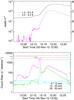 |
Fig. 1 Top panel: GOES time profiles of the C4.9 flare in two wavelengths (1–8 and 0.5–4.0 Å). Bottom panel: RHESSI time profiles of the same flare at different energy bands. |
We present here the observations of the GOES C4.9 class flare on 2010 November 3 associated with a CME from the NOAA active region 11121. The active region was located at S21E88 on that day on the solar disk. According to GOES observations, the flare was initiated at 12:07 UT, peaked at 12:15 UT, and ended around 12:30 UT. The flare or eruption was clearly observed by SDO/AIA at different wavelengths with high spatial (0.6 arcsec) and temporal resolution (12 s) as well as by the Reuven Ramaty High-Energy Solar Spectroscopic Imager (RHESSI, Lin et al. 2002) in X-ray 3–6 keV, 6–12 keV, 12–25 keV, and 25–50 keV energy bands. The temporal evolution of the flare in X-rays observed by GOES and RHESSI is presented in Fig. 1.
The SDO/AIA observations on 2010 November 3 at different wavelengths show evidence of a KH instability around 12:15 UT at 131 Å (see also Foullon et al. 2011, 2013). Figure 2 (top panel) shows the SDO/AIA 131 Å at 12:15 UT, where we can see the KH instability features (see the white rectangular box). The image is overlaid by the RHESSI 6–12 keV contours. The RHESSI image is constructed from seven collimators (3F to 9F) using the CLEAN algorithm, which yields a spatial resolution of ~7 arcsec (Hurford et al. 2002).
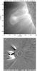 |
Fig. 2 Top panel: SDO/AIA 131 Å image overlaid by RHESSI X-ray contours (contour level: 40%, 70%, and 95% of the peak intensity). The rectangular white box shows where the KH instability is visible. Bottom panel: the associated difference image of the LASCO CME overlaid on the SDO/AIA image. |
LASCO observed a CME at 12:36 UT in the C2 field of view with a speed of 241 km s-1 and an angular width of 66° associated with the flare. The difference LASCO C2 images overlaid on the SDO 193 Å difference image is presented in the bottom panel of Fig. 2. In this image, some step-like structure is also visible, which corresponds to KH instability features visible in the SDO 131 Å wavelengths. This CME image shows that we can see the KH instability features up to a ~3 R⊙ height.
The study by Foullon et al. (2013) of the dynamics and origin of the CME on 2010 November 3 by means of the Solar TErrestrial RElations Observatory Behind (STEREO-B) located eastward of SDO by 82° of heliolongitude, and used in conjunction with SDO, gives some indication of the magnetic field topology and flow pattern. At the time of the event, the Extreme Ultraviolet Imager (EUVI) from STEREO’s Sun–Earth Connection Coronal and Heliospheric Investigation (SECCHI) instrument suite (Howard et al. 2008) achieved the highest temporal resolution in the 195 Å bandpass: EUVI’s images of the active region on the disk were taken every 5 min in this bandpass. The authors applied differential emission measure (DEM) techniques on the edge of the ejecta to determine the basic plasma parameters – they obtained an electron temperature of 11.6 ± 3.8 MK and an electron density of n = (7.1 ± 1.6) × 108 cm-3, together with a layer width ΔL = 4.1 ± 0.7 Mm. Density estimates of the ejecta environment (quiet corona), according to Aschwanden & Acton (2001), vary from (2 to 1) × 108 cm-3 between 0.05 and 0.15R⊙ (40–100 Mm), at heights where Foullon et al. (2013) started to see developing KH waves. The final estimate based on a maximum height of 250 Mm and the highest DEM value on the northern flank of the ejecta yields an electron density of (7.1 ± 0.8) × 108 cm-3. The adopted electron temperature in the ambient corona is T = 4.5 ± 1.5 MK. The other important parameters derived from using the pressure balance equation assuming a benchmark value for the magnetic field B in the environment of 10 G are summarized in Table 2. The main features of the imaged KH instability presented in Table 3 include (in their notation) the speed of the 131 Å CME leading edge, VLE = 687 km s-1, the flow shear on the 131 Å CME flank, V1 − V2 = 680 ± 92 km s-1, the KH group velocity, vg = 429 ± 8 km s-1, the KH wavelength, λ = 18.5 ± 0.5 Mm, and an exponential linear growth rate, γKH = 0.033 ± 0.012 s-1.
3. Geometry, the governing equations, and the wave dispersion relation
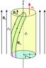 |
Fig. 3 Magnetic field geometry of a coronal mass ejection. Picture credit to Erdélyi & Fedun (2010). |
CMEs are ejections of magnetized plasma from the solar corona. Recently, Vourlidas (2014) presented observational evidence for the existence of magnetic flux ropes within CMEs. The observations detect the formation of the flux rope in the low corona, reveal its sometimes extremely fast evolution, and follow it into interplanetary space. The results validate many of the expectations of the CME initiation theories. The idea that the formation of magnetic flux ropes is associated with CMEs is not new. Manchester IV et al. (2005), who studied CME shocks and sheath structures relevant to particle acceleration in the solar wind by means of a three-dimensional numerical ideal MHD model, drove a CME to erupt by introducing a Gibson-Low magnetic flux rope that is embedded in the helmet streamer in an initial state of force imbalance. The flux rope rapidly expands and is ejected from the corona with maximum speeds in excess of 1000 km s-1, driving a fast-mode shock from the inner corona to a distance of 1 AU. Kumar et al. (2012) presented multi-wavelength observations of a helical kink instability as a trigger of a CME that occurred in active region NOAA 11163 on 2011 February 24 and stated that the high-resolution observations from the SDO/AIA suggest that the helical kink instability developed in the erupting prominence, which implies a flux rope structure of the magnetic field (see also Srivastava et al. 2010 for an observed kink instability in the solar corona). A brightening starts below the apex of the prominence with its slow rising motion (~100 km s-1) during the activation phase. In his review of recent studies on coronal dynamics such as streamers, CMEs, and their interactions, Chen (2013) claimed that the energy release mechanism of CMEs can be explained through a flux rope magnetohydrodynamic model. According to him, the rope is formed through a long-term reconnection process driven by the shear, twist, and rotation of magnetic footpoints; moreover, recent SDO studies discovered solar tornadoes providing a natural mechanism of rope formation (see, e.g., Zhang & Liu 2011; Li et al. 2012; Wedemeyer-Böhm et al. 2012). Recent in situ measurements also suggest that the twisted magnetic tubes might be common in the solar wind (Zaqarashvili et al. 2014b). Thus, we are convinced to accept the expanded definition of the CME suggested in Vourlidas et al. (2013): “a CME is the eruption of a coherent magnetic, twist-carrying coronal structure with angular width of at least 40° and able to reach beyond 10 R⊙ which occurs on a time scale of a few minutes to several hours.” Accordingly, the most appropriate model of the CME under consideration is a twisted magnetic flux tube of radius a (= ΔL/ 2) and density ρi embedded in a uniform field environment with density ρe (see Fig. 3). The magnetic field inside the tube is helicoidal, Bi = (0,Biϕ(r),Biz(r)), while on the outside it is uniform and directed along the z-axis, Be = (0,0,Be). The tube moves along its axis with a velocity of v0 with regard to the surrounding medium. The jump of the tangential velocity at the tube boundary then triggers the magnetic KH instability when the jump exceeds a critical value.
In cylindrical equilibrium the magnetic field and plasma pressure satisfy the equilibrium condition in the radial direction 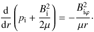 (1)Here,
  denotes the strength of the equilibrium magnetic field and μ is the magnetic permeability. We note that in Eq. (1) the total (thermal plus magnetic) pressure gradient is balanced by the tension force (the right-hand side of Eq. (1)) in the twisted field. We consider the special case of an equilibrium with uniform twist, that is, the one for which Biϕ(r) /rBiz(r) is a constant. Thus the background magnetic field is assumed to be
 ![Mathematical equation: \begin{equation} \label{eq:magnfield} {\vec B}(r) = \left\{ \begin{array}{lc} (0, Ar, B_{{\rm i} z}) & ~~~{\rm for}~~~ r \leqslant a, \\[1mm] (0, 0, B_{\rm e}) & ~~~{\rm for}~~~ r > a, \end{array} \right. \end{equation}](/articles/aa/full_html/2015/02/aa24793-14/aa24793-14-eq70.png) (2)where A, Biz, and Be are constant. Then the equilibrium condition (1) gives the equilibrium plasma pressure pi(r) as
(2)where A, Biz, and Be are constant. Then the equilibrium condition (1) gives the equilibrium plasma pressure pi(r) as
 where p0 is the plasma pressure at the centre of the tube. We note that the jump in the value of Bϕ(r) across r = a implies a surface current there.
Before starting with governing MHD equations, we specify what kind of plasma each medium is (the moving tube and its environment). The CME parameters listed in Table 2 in Foullon et al. (2013) show that the plasma beta inside the flux tube might be equal to 1.5 ± 1.01, while that of the coronal plasma is 0.21 ± 0.05. Hence, we can consider the ejecta as an incompressible medium and treat its environment as a cool plasma (βe = 0).
The plasma motion inside the twisted flux tube is governed by the set of linearised MHD equations for an ideal incompressible plasma: 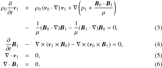
Here, the index “0” denotes equilibrium values of the fluid velocity and the medium magnetic field, and the index “1” their perturbations. Below, the sum p1 + B0·B1/μ in Eq. (3) is replaced by p1tot, which represents the total pressure perturbation.
As the unperturbed parameters only depend on the r coordinate, the perturbations can be Fourier analysed with exp[i(−ωt + mϕ + kzz)]. Bearing in mind that in cylindrical coordinates the nabla operator has the form
 from the above set of equations one can obtain a second-order differential equation for the total pressure perturbation p1tot
![Mathematical equation: \begin{equation} \label{eq:diffeq} \left[ \frac{\mathrm{d}^2}{\mathrm{d}r^2} + \frac{1}{r} \frac{\mathrm{d}}{\mathrm{d} r} - \left( \kappa_{\rm i}^2 + \frac{m^2}{r^2} \right) \right] p_{\rm 1 tot} = 0, \end{equation}](/articles/aa/full_html/2015/02/aa24793-14/aa24793-14-eq90.png) (7)as well as an expression for the radial component v1r of the fluid velocity perturbation v1 in terms of p1tot and its first derivative
(7)as well as an expression for the radial component v1r of the fluid velocity perturbation v1 in terms of p1tot and its first derivative  (8)In Eq. (7), κi is the so-called wave attenuation coefficient, which characterises the space structure of the wave and whose squared magnitude is given by the expression
 ![Mathematical equation: \begin{equation} \label{eq:kappa} \kappa_{\rm i}^2 = k_z^2 \left( 1 - \frac{4 A^2 \omega_{\rm Ai}^2} {\mu \rho_{\rm i} \left[ \left( \omega - {\vec k} \cdot {\vec v}_0 \right)^2 - \omega_{\rm Ai}^2\right]^2} \right), \end{equation}](/articles/aa/full_html/2015/02/aa24793-14/aa24793-14-eq95.png) (9)where
(9)where  (10)is the so-called local Alfvén frequency (Bennett et al. 1999). The numerical coefficients Z and Y in the expression of v1r (see Eq. (8)) are
![Mathematical equation: $$ Z = \frac{2A \omega_{\rm Ai}}{\sqrt{\mu \rho_{\rm i}}\left[ \left( \omega - {\vec k} \cdot {\vec v}_0 \right)^2 - \omega_{\rm Ai}^2\right]} \qquad \mbox{and} \qquad Y = 1 - Z^2. $$](/articles/aa/full_html/2015/02/aa24793-14/aa24793-14-eq99.png) The solution to Eq. (7) bounded at the tube axis is
The solution to Eq. (7) bounded at the tube axis is  (11)where Im is the modified Bessel function of order m and αi is a constant.
For the cool environment (thermal pressure pe = 0) with straight-line magnetic field Bez = Be and homogeneous density ρe, from governing Eqs. (3), (4), and (6), in a similar way the same modified Bessel Eq. (7) is obtained, but  is replaced by
  (12)where
  (13)and
  is the Alfvén speed in the corona. The solution to the modified Bessel equation bounded at infinity is
  (14)where Km is the modified Bessel function of order m and αe is a constant.
From Eq. (3), written down for the radial components of all perturbations, we obtain that
 or
or  (15)where the prime sign means a differentiation by the Bessel function argument.
To obtain the dispersion relation of MHD modes, we merge the solutions for ptot and v1r inside and outside the tube through boundary conditions. The boundary conditions have to ensure that the normal component of the interface perturbation
 remains continuous across the unperturbed tube boundary r = a, and also that the total Lagrangian pressure is conserved across the perturbed boundary. This leads to the conditions (Bennett et al. 1999)
 (16)and
  (17)where total pressure perturbations ptot i and ptot e are given by Eqs. (11) and (14), respectively. Applying boundary conditions (16) and (17) to our solutions of p1tot and v1r (and accordingly ξr), we obtain after some algebra the dispersion relation of the normal modes propagating along a twisted magnetic tube with axial mass flow v0
![Mathematical equation: \begin{eqnarray} \label{eq:dispeq} \frac{\left[ \left( \omega - {\vec k}\cdot {\vec v}_0 \right)^2 - \omega_{\rm Ai}^2 \right]F_m(\kappa_{\rm i}a) - 2mA \omega_{\rm Ai}/\sqrt{\mu \rho_{\rm i}}} {\left[ \left( \omega - {\vec k}\cdot {\vec v}_0 \right)^2 - \omega_{\rm Ai}^2 \right]^2 - 4A^2\omega_{\rm Ai}^2/\mu \rho_{\rm i} } =\nonumber \\ \nonumber \\ {} \frac{P_m(\kappa_{\rm e} a)} {{\displaystyle \frac{\rho_{\rm e}}{\rho_{\rm i}}} \left( \omega^2 - \omega_{\rm Ae}^2 \right) + A^2 P_m(\kappa_{\rm e} a)/\mu \rho_{\rm i}}, \end{eqnarray}](/articles/aa/full_html/2015/02/aa24793-14/aa24793-14-eq121.png) (18)where, ω − k·v0 is the Doppler-shifted wave frequency in the moving medium, and
(18)where, ω − k·v0 is the Doppler-shifted wave frequency in the moving medium, and
 This dispersion equation is similar to the dispersion equation of normal MHD modes in a twisted flux tube surrounded by incompressible plasma (Zhelyazkov & Zaqarashvili 2012 – there, in Eq. (13), κe = kz), and to the dispersion equation for a twisted tube with non-magnetized environment, that is, with ωAe = 0 (Zaqarashvili et al. 2010).
4. Numerical solutions and wave dispersion diagrams
The main goal of our study is to determine under which conditions the MHD waves propagating along the moving flux tube can become unstable. To conduct this investigation, it is necessary to assume that the wave frequency ω is a complex quantity, that is, ω → ω + iγ, where γ is the instability growth rate, while the longitudinal wave number kz is a real variable in the wave dispersion relation. Since the occurrence of the expected KH instability is determined primarily by the jet velocity, by searching for a critical or threshold value of it, we will gradually change its magnitude from zero to that critical value (and beyond). Thus, we have to solve dispersion relations in complex variables, obtaining the real and imaginary parts of the wave frequency, or as is commonly accepted, of the wave phase velocity vph = ω/kz, as functions of kz at various values of the velocity shear between the surge and its environment, v0.
We focus our study first on the propagation of the kink mode, m = 1. It is obvious that Eq. (18) can only be solved numerically. The necessary step is to define the input parameters that characterise the moving twisted magnetic flux tube and also normalise all variables in the dispersion equation. The density contrast between the tube and its environment is characterised by the parameter η = ρe/ρi and the twisted magnetic field by the ratio of the two magnetic field components, Biϕ and Biz, evaluated at the inner boundary of the tube, r = a, that is, via ε = Biϕ/Biz, where Biϕ = Aa. As usual, we normalise the velocities to the Alfvén speed vAi = Biz/ (μρi)1/2. Thus, we introduce the dimensionless wave phase velocity vph/vAi and the Alfvén Mach number MA = v0/vAi, the latter characterising the axial motion of the tube. The wavelength, λ = 2π/kz, is normalised to the tube radius a , which implies that the dimensionless wave number is kza. The natural way of normalising the local Alfvén frequency ωAi is to multiply it by the tube radius, a, and after that divide by the Alfvén speed vAi, that is,
 where Biϕ/Biz ≡ Aa/Biz = ε is the twist parameter defined above. We note that the normalisation of the Alfvén frequency outside the jet, ωAe, requires (see Eq. (13)) in addition to the tube radius, a, and the density contrast, η, the ratio of the two axial magnetic fields, b = Be/Biz.
Before starting the numerical task, we specify the values of the input parameters. Our choice for the density contrast is η = 0.88, which corresponds to electron densities ni = 8.7 × 108 cm-3 and ne = 7.67 × 108 cm-3. With βi = 1.5 and βe = 0, the ratio of axial magnetic fields is b = 1.58. If we fix the Alfvén speed in the environment to be vAe ≅ 787 km s-1 (i.e., the value corresponding to ne = 7.67 × 108 cm-3 and Be = 10 G), the total pressure balance equation at η = 0.88 requires a sound speed inside the jet of csi ≅ 523 km s-1 and an Alfvén speed vAi ≅ 467 km s-1 (more exactly, 467.44 km s-1), which corresponds to a magnetic field in the flux tube Biz = 6.32 G. Following Ruderman (2007), to satisfy the Shafranov-Kruskal stability criterion for a kink instability, we assume that the azimuthal component of the magnetic field Bi is smaller than its axial component, meaning that we choose our twist parameter ε to be always lower than 1. In particular, we study the dispersion diagrams of kink, m = 1 and m = −3 MHD modes and their growth rates (when the modes are unstable) for three fixed values of ε: 0.025, 0.1, and 0.2.
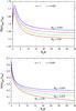 |
Fig. 4 Top panel: dispersion curves of an unstable kink (m = 1) mode propagating on a moving twisted magnetic flux tube with twist parameter ε = 0.025 at η = 0.88, b = 1.58 and Alfvén Mach numbers equal to 2.95, 2.975, 3, and 3.025. Bottom panel: growth rates of the unstable kink mode. Note that the marginal red curve reaches values lower than 0.001 beyond kza = 53. |
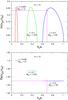 |
Fig. 5 Top panel: growth rates of an unstable m = −3 MHD mode in three instability windows. Adequate numerical values consistent with the observational data are obtained at kza = 0.696245, located in the third instability window, for which value of the dimensionless wave number the normalised mode growth rate is equal to 0.232117. Bottom panel: dispersion curves of unstable m = −3 MHD mode for three values of the twist parameter ε = 0.025, 0.1, and 0.2. The normalised phase velocity at kza = 0.696245 is equal to 1.45. |
With these input parameters (MA is varied from zero (no flow) to reasonable values during computations), the solutions to Eq. (18) yield the dependence of the normalised wave phase velocity ω/kzvAi on kza. In Fig. 4 we display the dispersion curves of the kink mode at ε = 0.025 for various values of MA – the red curve is in fact a marginal dispersion curve corresponding to the critical  . The critical jet speed,
  km s-1, which in principle is accessible for CMEs, is, in fact, more than twice as high as the speed registered by Foullon et al. (2013), who reported a threshold speed of 680 km s-1 for observing a KH instability. For the next higher values of ε, threshold Alfvén Mach numbers of about 3 are obtained. Hence, the detected KH instability cannot be associated with the kink mode. But the situation distinctly changes for the m = −3 MHD mode. Figure 5 shows the appearance of three instability windows on the kza-axis. The width of each instability window depends upon the value of the twist parameter ε – the narrowest window corresponds to ε = 0.025, and the widest to ε = 0.2. The phase velocities of unstable m = −3 MHD modes coincide with the magnetic flux tube speeds (the bottom panel of Fig. 5 shows that the normalised wave velocity on a given dispersion curve is equal to its label MA). Therefore, unstable perturbations are frozen in the flow, and consequently, they are vortices rather than waves. This is firmly based on physics because the KH instability in hydrodynamics deals with unstable vortices. All critical Alfvén Mach numbers yield acceptable threshold speeds of the ejecta that ensure the occurrence of KH instability – these speeds are equal to 701 km s-1, 689 km s-1, and 678 km s-1 and agree very well with the speed of 680 km s-1 found by Foullon et al. (2013). The observationally detected KH instability wavelength λKH = 18.5 Mm and ejecta width ΔL = 4.1 Mm define the corresponding instability dimensionless wave number, kza = πΔL/λ, to be equal to 0.696245. Figure 5 shows that kza = 0.696245 lies in the third instability window and accordingly determines a value of the dimensionless growth rate Im(vph/vAi) = 0.232117 (see the top panel of Fig. 5), which implies a computed wave growth rate γKH = 0.037 s-1, being in good agreement with the deduced from observations γKH = 0.033 s-1. We also note that the wave phase velocity estimated from Fig. 5 (bottom panel) of 678 km s-1 is rather close to the speed of the 131 Å CME leading edge, which is equal to 687 km s-1. The position of a given instability window, at fixed input parameters η and b, is determined chiefly by the magnetic field twist in the moving flux tube. This circumstance allows us by slightly shifting the third instability window to the right, to tune the vertical purple line (see the top panel of Fig. 5) to cross the growth rate curve at a value that would yield γKH = 0.033 s-1. The necessary shift of only 0.023625 can be achieved by taking the magnetic field twist parameter, ε, to be equal to 0.20739 – in that case, the normalised Im(vph/vAi) = 0.207999 gives the registered KH instability growth rate of 0.033 s-1. (That very small instability window shift does not change the critical ejecta speed by much.) In this way, we demonstrate the flexibility of our model, which allows deriving the numerical KH instability characteristics in very good agreement with observational data.
5. Discussion and conclusion
The KH vortices imaged by Foullon et al. (2013) on the 2010 November 3 CME can be explained as a KH instability of the m = −3 harmonic in a twisted flux tube moving in external cool magnetized plasma embedded in a homogeneous untwisted magnetic field. We have assumed the wave vector k to be aligned with the v0 = Vi − Ve vector. We would like to point out that the results of the numerical modelling crucially depend on the input parameters. Any small change in the density contrast, η, or the magnetic fields ratio, b, can dramatically change the picture. In our case, the input parameters for solving the MHD mode dispersion relation in complex variables (the mode frequency ω and, respectively, the mode phase velocity vph = ω/kz, were considered as complex quantities) were chosen to be consistent with the plasma and magnetic field parameters listed in Table 2 in Foullon et al. (2013). With a twist parameter of the background magnetic filed Bi, ε = 0.2, the critical jet speed is  km s-1, and at a wavelength of the unstable m = −3 mode λKH = 18.5 Mm and ejecta width ΔL = 4.1 Mm, its growth rate is γKH = 0.037 s-1. These values of
  and γKH agree well with the data listed in Table 3 of Foullon et al. (2013). We also showed that the numerically obtained instability growth rate can be slightly reduced to coincide with the observational rate of 0.033 s-1 through slightly shifting the appropriate instability window to the right – this can be done by performing the calculations with a new value of the magnetic field twist parameter ε, equal to 0.20739. Thus, our model is flexible enough to allow us to numerically derive KH instability characteristics very close to the observed ones. The two “cross points” in Fig. 5 can be considered as a “computational portrait” of the coronal mass ejecta KH instability imaged on 2010 November 3. Critical ejecta speed and KH instability growth rate values, in good agreement with those derived by Foullon et al. (2013), can also be obtained by exploring the fluting-like, m = −2, MHD mode (Zhelyazkov & Chandra 2014). In that case, a better agreement with the observational data is achieved at ε = 0.188 – the computed values of and γKH are exactly the same as those for the m = −3 mode.
We stress that each CME is a unique event, and modelling it successfully requires a full set of observational data for the plasma densities, magnetic fields, and temperatures of both media along with the detected ejecta speeds. The flux tube speeds at which the instability starts can vary from a few kilometers per second, 6–10 km s-1, as observed by Ofman & Thompson (2011), through 310 ± 20 km s-1 as reported by Möstl et al. (2013), to 680 ± 92 km s-1 deduced from Foullon et al. (2013). It would be interesting to investigate whether the 13 fast flareless CMEs (with velocities of 1000 km s-1 and higher) observed from 1998 January 3 to 2005 January 4 (see Table 1 in Song et al. 2013) are subject to the KH instability.
Although the KH instability characteristics of both m = −2 and m = −3 MHD modes agree well with observational data, only the instability of the m = −3 harmonic may explain why the KH vortices are seen only at one side of rising CME (Foullon et al. 2011; 2013, see also Fig. 2 in the present paper). This harmonic yields that the unstable vortices have three maxima around the magnetic tube with a 360/3 = 120 degree interval. Therefore, if one maximum is located in the plane perpendicular to the line of sight (as it is clearly seen by observations), then one cannot detect two other maxima in imaging observations because they will be largely directed along the line of sight.
Finally, we would like to comment on whether there is a required field orientations  . From analysing a flat (semi-infinite) geometry in their study, Foullon et al. (2013) concluded that it is most probable to observe a wave propagation quasi-perpendicular to the magnetic field Be. But this restriction on the ejecta magnetic field tilt angle cancels out in our numerical investigation because the inequality
  km s-1, required for wave parallel propagation, is satisfied. Thus, the adopted magnetic flux rope nature of a CME and its (ejecta) consideration as a moving twisted magnetic flux tube allow us to explain the emerging instability as a manifestation of the KH instability of a suitable MHD mode.
Acknowledgments
The work of two of us, I.Zh. and R.C., was supported by the Bulgarian Science Fund and the Department of Science & Technology, Government of India Fund under Indo-Bulgarian bilateral project CSTC/INDIA 01/7, /Int/Bulgaria/P-2/12. The work of T.Z. was supported by the European FP7-PEOPLE-2010-IRSES-269299 project- SOLSPANET, by the Austrian Fonds zur Förderung der Wissenschaftlichen Forschung (project P26181-N27) and by Shota Rustaveli National Science Foundation grant DI/14/6-310/12 and by Austrian Scientific-technology collaboration (WTZ) grant IN 10/2013. We would like to thank the referee for the very useful comments and suggestions that helped us improve the quality of our paper, and we are indebted to Snezhana Yordanova for drawing one figure.
References
- Aschwanden, M. J., & Acton, L. W. 2001, ApJ, 550, 475 [NASA ADS] [CrossRef] [Google Scholar]
- Aulanier, G. 2014, in Nature of Prominences and their role in Space Weather, eds. B. Schmieder, J.-M. Malherbe, & S. T. Wu (New York: Cambridge University Press), Proc. IAU Symp., 300, 184 [Google Scholar]
- Aulanier, G., Török, T., Démoulin, P., & DeLuca, E. E. 2010, ApJ, 708, 314 [Google Scholar]
- Bennett, K., Roberts, B., & Narain, U. 1999, Sol. Phys., 185, 41 [NASA ADS] [CrossRef] [Google Scholar]
- Brueckner, G. E., Howard, R. A., Koomen, M. J., et al. 1995, Sol. Phys., 162, 357 [NASA ADS] [CrossRef] [Google Scholar]
- Chandra, R., Schmieder, B., Mandrini, C. H., et al. 2011, Sol. Phys., 269, 83 [NASA ADS] [CrossRef] [Google Scholar]
- Chandrasekhar, S. 1961, Hydrodynamic and Hydromagnetic Stability (Oxford: Clarendon Press) [Google Scholar]
- Chen, Y. 2013, Chin. Sci. Bull., 58, 1599 [CrossRef] [Google Scholar]
- DeanPesnell, W., Thompson, B. J., & Chamberlin, P. C. 2012, Sol. Phys., 275, 3 [NASA ADS] [CrossRef] [Google Scholar]
- Drazin, P. G., & Reid, W. H. 1981, Hydrodynamic Stability (Cambridge: Cambridge University Press) [Google Scholar]
- Forbes, T. G., Linker, J. A., Chen, J., et al. 2006, Space Sci. Rev., 123, 251 [NASA ADS] [CrossRef] [Google Scholar]
- Foullon, C., Verwichte, E., Nakariakov, V. M., Nykyri, K., & Farrugia, C. J. 2011, ApJ, 729, L8 [NASA ADS] [CrossRef] [Google Scholar]
- Foullon, C., Verwichte, E., Nykyri, K., Aschwanden, M. J., & Hannah, I. G. 2013, ApJ, 767, 170 [NASA ADS] [CrossRef] [Google Scholar]
- Howard, T. A., Moses, J. D., Vourlidas, A., et al. 2008, Space Sci. Rev., 136, 67 [NASA ADS] [CrossRef] [Google Scholar]
- Hurford, G. J., Schmahl, E. J., Schwartz, R. A., et al. 2002, Sol. Phys., 210, 61 [NASA ADS] [CrossRef] [Google Scholar]
- Kumar, P., Cho, K.-S., Bong, S.-C., Sung-Hong, Park, & Kim, Y. H. 2012, ApJ, 746, 67 [NASA ADS] [CrossRef] [Google Scholar]
- Lemen, J. R., Title, A. M., Akin, D. J., et al. 2012, Sol. Phys., 275, 11 [Google Scholar]
- Li, X., Morgan, H., Leonard, D., et al. 2012, ApJ, 752, L22 [NASA ADS] [CrossRef] [EDP Sciences] [Google Scholar]
- Lin, R. P., Dennis, B. R., Hurford, G. J., et al. 2002, Sol. Phys., 210, 3 [Google Scholar]
- Manchester IV, W. B., Gombosi, T. I., De Zeeuw, D. L., et al. 2005, ApJ, 622, 1225 [NASA ADS] [CrossRef] [Google Scholar]
- Möstl, U. V., Temmer, M., & Veronig, A. M. 2013, ApJ, 766, L12 [NASA ADS] [CrossRef] [Google Scholar]
- Ofman, L., & Thompson, B. J. 2011, ApJ, 734, L11 [NASA ADS] [CrossRef] [Google Scholar]
- Ruderman, M. S. 2007, Sol. Phys., 246, 119 [NASA ADS] [CrossRef] [Google Scholar]
- Sakurai, T. 1976, PASJ, 28, 177 [NASA ADS] [Google Scholar]
- Schmieder, B., Démoulin, P., & Aulanier, G. 2013, Adv. Space Res., 51, 1967 [NASA ADS] [CrossRef] [Google Scholar]
- Song, H. Q., Chen, Y., Ye, D. D., Han, G. Q., et al. 2013, ApJ, 773, 129 [NASA ADS] [CrossRef] [Google Scholar]
- Srivastava, A. K., Zaqarashvili, T. V., Kumar, P., & Khodachenko, M. L. 2010, ApJ, 715, 292 [NASA ADS] [CrossRef] [Google Scholar]
- Török, T., & Kliem, B. 2005, ApJ, 630, L97 [Google Scholar]
- Vourlidas, A. 2014, Plasma Phys. Control. Fusion, 56, 064001 [NASA ADS] [CrossRef] [Google Scholar]
- Vourlidas, A., Lynch, B. J., Howard, R. A., & Li, Y. 2013, Sol. Phys., 284, 179 [NASA ADS] [Google Scholar]
- Webb, D. F., & Howard, T. A. 2012, Liv. Rev. Sol. Phys., 9, 3 [Google Scholar]
- Wedemeyer-Böhm, S., Scullion, E., Steiner, O., et al. 2012, Nature, 486, 505 [NASA ADS] [CrossRef] [PubMed] [Google Scholar]
- Zaqarashvili, T. V., Díaz, A. J., Oliver, R., & Ballester, J. L. 2010, A&A, 516, A84 [NASA ADS] [CrossRef] [EDP Sciences] [Google Scholar]
- Zaqarashvili, T. V., Vörös, Z., & Zhelyazkov, I. 2014a, A&A, 561, A62 [NASA ADS] [CrossRef] [EDP Sciences] [Google Scholar]
- Zaqarashvili, T. V., Vörös, Z., Narita, Y., & Bruno, R. 2014b, ApJ, 783, L19 [NASA ADS] [CrossRef] [Google Scholar]
- Zhang, J., & Liu, Y. 2011, ApJ, 741, L7 [NASA ADS] [CrossRef] [Google Scholar]
- Zhelyazkov, I., & Chandra, R. 2014, Compt. Rend. Acad. Bulg. Sci., 67, 1145 [Google Scholar]
- Zhelyazkov, I., & Zaqarashvili, T. 2012, A&A, 547, A14 [NASA ADS] [CrossRef] [EDP Sciences] [Google Scholar]
All Figures
|
Fig. 1 Top panel: GOES time profiles of the C4.9 flare in two wavelengths (1–8 and 0.5–4.0 Å). Bottom panel: RHESSI time profiles of the same flare at different energy bands. |
| In the text | |
|
Fig. 2 Top panel: SDO/AIA 131 Å image overlaid by RHESSI X-ray contours (contour level: 40%, 70%, and 95% of the peak intensity). The rectangular white box shows where the KH instability is visible. Bottom panel: the associated difference image of the LASCO CME overlaid on the SDO/AIA image. |
| In the text | |
|
Fig. 3 Magnetic field geometry of a coronal mass ejection. Picture credit to Erdélyi & Fedun (2010). |
| In the text | |
|
Fig. 4 Top panel: dispersion curves of an unstable kink (m = 1) mode propagating on a moving twisted magnetic flux tube with twist parameter ε = 0.025 at η = 0.88, b = 1.58 and Alfvén Mach numbers equal to 2.95, 2.975, 3, and 3.025. Bottom panel: growth rates of the unstable kink mode. Note that the marginal red curve reaches values lower than 0.001 beyond kza = 53. |
| In the text | |
|
Fig. 5 Top panel: growth rates of an unstable m = −3 MHD mode in three instability windows. Adequate numerical values consistent with the observational data are obtained at kza = 0.696245, located in the third instability window, for which value of the dimensionless wave number the normalised mode growth rate is equal to 0.232117. Bottom panel: dispersion curves of unstable m = −3 MHD mode for three values of the twist parameter ε = 0.025, 0.1, and 0.2. The normalised phase velocity at kza = 0.696245 is equal to 1.45. |
| In the text | |
Current usage metrics show cumulative count of Article Views (full-text article views including HTML views, PDF and ePub downloads, according to the available data) and Abstracts Views on Vision4Press platform.
Data correspond to usage on the plateform after 2015. The current usage metrics is available 48-96 hours after online publication and is updated daily on week days.
Initial download of the metrics may take a while.