| Issue |
A&A
Volume 574, February 2015
|
|
|---|---|---|
| Article Number | L2 | |
| Number of page(s) | 4 | |
| Section | Letters | |
| DOI | https://doi.org/10.1051/0004-6361/201424651 | |
| Published online | 12 February 2015 | |
Analysis of time series in space maser signals⋆
1 Department of Physics, State University of Civil Aviation, St.-Petersburg, Russia
e-mail: This email address is being protected from spambots. You need JavaScript enabled to view it.
2 National Research University of Information Technologies, Mechanics and Optics, St.-Petersburg, Russia
3 Radio Astronomy Observatory of Lebedev Physical Institute of the Russian Academy of Sciences, Pushchino, Russia
4 Teknavo Group, St.-Petersburg, Russia
Received: 22 July 2014
Accepted: 12 December 2014
Abstract
Many astrophysical sources that emit narrow radio-frequency spectral lines are believed to be sets of molecular condensation, each of which works as a maser, so that the whole set produces a characteristic spectrum. The forms of these spectra vary with time on various time-scales from months to dozens of minutes. We analysed the ultra-short variations of the separate components of space maser spectra in search for the periodical behaviour. We used a consecutive statistical analysis of the observation data that includes fast Fourier transformations (FFTs), a Lomb-Scargle procedure, and a modified Lomb-Scargle procedure. In at least 8 of the 49 sources we studied, we found that the intensity of one of the components of a space maser spectrum that corresponds to a single condensation changes periodically with a period of dozens of minutes or hours. Three sources had a period of 68 min; in one source the oscillations lasted at least four days.
Key words: gravitational waves / masers / binaries: close
FITS data are only available at the CDS via anonymous ftp to cdsarc.u-strasbg.fr (130.79.128.5) or via http://cdsarc.u-strasbg.fr/viz-bin/qcat?J/A+A/574/L2
© ESO, 2015
1. Introduction
Space masers are sources of almost monochromatic radiation that is produced by the dense condensations in the clouds of molecules in meta-stable states. This radiation can be registered by radio telescopes, and there are many known masers. The regions in clouds that provide maser radiation typically have diameters of 100−102 au (Reid & Morgan 1981), while the radiation spectra occupy the bands corresponding to the total velocity extent of 102 km s-1. The spectra contain series of narrow details that extend over 0.5−1.0 km s-1 at half-power level and correspond to condensations with typical sizes of 1 au or more. The condensations may have various densities and can move relative to one another (Imai et al. 2002). The origin of pumping may also vary for various masers; thus, the intensities of sub-au-details may vary with time too. The variability of masers in star-forming regions over months or years is widespread for methanol masers (Goedhart et al. 2014) and has been observed for water masers (Lekht & Munitsyn 2010), but intra-day variability has been reported very rarely. Samodurov et al. (2010) showed that there exist situations when the space maser radiation has ultra-rapid fluctuations (tens of minutes). This cannot be an instrumental, weather, or interstellar medium instability influence because it is a single detail of the spectrum that fluctuates and not the whole set of them. Therefore, the ultra-rapid variability is caused by a process inside the maser or by external action. For example, it can be explained by the competition between the close condensations for the radiation pumping; by the changes inside the condensations; by the fast superimpositions of the condensations over the line of sight; by the turbulence phenomena inside the maser, etc. We have also eliminated potential correlator or other channel-dependent instrumental artefacts, and there is no known radio interference in this band. It was also found (Siparov & Samodurov 2009) that there exist situations when the intensity variation for a single spectrum detail has a periodic character and provides several periods per observational session. At the same time, the other details of the spectrum do not show a similar behaviour (at least visually) during the session. As before, this peculiar behaviour excludes an instrumental, weather, or interstellar medium effect. Therefore, it seemed reasonable to investigate the corresponding time dependencies for various space masers.
2. Observations, data preparation, and analysis
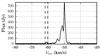 |
Fig. 1 Maser W3(OH): RA = 2h23m18s, Dec = 61°38′58′′, Dist ~2000 pc (RT-22, June 30, 2009, Puschino RAO RAS). |
In the years 2002 to 2009, we monitored 49 maser sources 2–5 times each during about 150 observational sessions. The observations were focused mostly on the 22 GHz water masers and one hydroxyl maser W3(OH). A single observation session typically lasted several hours. At short intervals, the gathered spectrum was transferred to the recorder, and we constructed the dependence of the flux intensity (Jy km s-1) at a given frequency on the value of this frequency (more precisely, on the detuning of the given frequency from the main one). The observations at λ = 1.35 cm were carried out on RT-22 (the 22-m radio telescope of the Pushchino Radio Astronomy Observatory of Lebedev Physical Institute, Russian Academy of Sciences) in a number of observational sessions. Some of the masers varied on scales of tens of minutes. To perform the spectral analysis, we used the signal from the 2048-channel auto-correlator with a total bandwidth of 12.5 MHz (168.5 km s-1) and with a velocity resolution of 0.082 km s-1 corresponding to one channel. In the beginning of the observational session, the velocity data were corrected for the motion of Earth and sent to LSR. Various spectra had various small daily shifts (mainly due to the daily rotation of Earth), but they gave not more than 200 m s-1 per session and were shorter than the range of data counts for a single spectral feature. The RT-22 has two spaced receivers in dish focus, and similarly to Samodurov et al. (2010), the observations were performed in two ways:
-
1.
The signal was gathered from a place without sources; then thecalibration was performed for this empty place. After that, thesignal from the source was measured on the first receiver (positivevoltage) and then on the second receiver (negative voltage). Thismethod produces very accurate data, but it has a very large timespan and one spectrum can be obtained in not less than2 min.
-
2.
The signal was gathered from a place without sources; then the calibration was performed for this empty place. After that, the first receiver (positive voltage) measured N spectra (from 10 to 1000). The calibration took about five minutes, and then the spectra with 1 to 60 s expositions had been measured for half an hour. After that, the calibration-measurement cycle was repeated. This method was used most frequently.
The dedicated modernised registration channel of the telescope enabled gathering data for the accumulation period equal to 30 s. Every half hour during the session, the observations were interrupted for five minutes to calibrate the antenna. The preliminary stage of the signal processing included control of the antenna and registering channel. The special program designed for processing of the obtained data performed the rest. First, this program sums the flux values for the corresponding frequencies for all the spectra obtained during the given session and determines the frequencies corresponding to all the local minima in this sum. Then it takes every region between the neighbouring minima (e.g. see the detail between the dashed lines in Fig. 1) for every flux spectrum of the given observation session, follows its change with time, and produces the corresponding time series for this region, as shown in Fig. 2. The analysis of the time series includes three stages: FFT, which is used to discover whether there is a periodic component, this corresponds to a solitary peak in the plot, as shown in Fig. 3; Lomb-Scargle (LS) procedure, which exploits a more complicated algorithm (Lomb 1976; Scargle 1982) to construct a periodogram, a plot with a set of peaks corresponding to the periodic components, as shown in Fig. 4; and, finally, the generalized LS algorithm (Zechmeister & Kurster 2009; Ivezić et al. 2014), which filters out the periodic features that characterize the observation procedure itself, shown in Fig. 5. The FFT was previously used in Siparov & Samodurov (2009) to give the objective evidence that periodic components do exist in the space maser signals, but this approach is limited because it only deals with equidistant points and requires some interpolation.
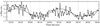 |
Fig. 2 Time dependence of the selected detail shown in Fig. 1. |
The periodogram in Fig. 4 shows several peaks, but some of them could be due to the total time of the session, to the period of antenna calibration, and to the number of measurements between calibrations (Vitiazev 2001). The high peak in Fig. 5 presents a period of 68 min corresponding to the non-stationary component of the selected maser signal detail marked in Fig. 1. None of the other details of the spectrum in Fig. 1 changes periodically, nor do they lead to a peak like that in Fig. 5. Therefore, this peak characterizes the periodical change of the radiation intensity emitted by only one of the condensations that form the space maser cloud.
The periodic behaviour of this source detail is not always present. For W3(OH), for example, the periodicity was registered in 5 out of 16 sessions. Two of them gave one and the same period equal to 68 min. This could mean that if the cause of the periodic behaviour is external to the maser cloud system, the radiation can still be affected by the dynamical situation inside the cloud. Figure 6 shows the 68 min peak obtained by a similar analysis for the observation session four days before the session illustrated in the previous figures.
To determine the phase coincidence between the signals registered on June 26 and June 30, the corresponding time dependencies were approximated by the sine functions with the help of a Levenberg-Marquardt algorithm (Levenberg 1944; Marquardt 1963). Then the time difference (in minutes) between a maximum approximating the plot in Fig. 2 and a maximum in the corresponding plot for June 26 session was divided by 68. The result was an integer within the accuracy of 0.029. This indicates that there is one and the same cause acting on the maser region and providing both 68 min peaks. In addition, in three other sessions with W3(OH), one session had another spectrum detail that changed with a period of 84 min.
Signals like the one plotted in Fig. 5 were also found for the following sources: Cep A, IRAS 16293-2422, Ori A, RT Vir, W 49 N, W 31 A, W 3(2), and VY CMa. The periods of the periodic components in these sources vary from 50 to 120 min, but no correlations between them were found. But the period equal to 68 min was found in two of them. These are space masers Cep-A (Figs. 7 and 8) and W 3(2) (Figs. 9 and 10).
3. Conclusions
-
1.
Our analysis of the time series in the space maser signals showsthat in the spectrum of some masers there are components thatvary with time periodically with periods of dozens of minutes,while other components of the spectrum demonstrate no suchbehaviour.
-
2.
A variation with a period equal to 68 min was found for W3(OH), Cep A, and W 3(2).
-
3.
For W3(OH), these periodic variations were registered twice during the subsequent sessions in four days, and they appeared to be correlated.
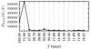 |
Fig. 3 Preliminary FFT analysis of the dependence on time of the power spectrum density for the feature marked in Fig. 1. |
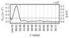 |
Fig. 5 Generalized Lomb-Scargle periodogram for the power spectrum density for the feature marked in Fig. 1; ΔBIC is the Bayesian information criterion; the dotted lines show the 1% and 5% significance levels. |
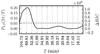 |
Fig. 6 Generalized Lomb-Scargle periodogram for the power spectrum density for maser W3(OH): RA = 2h23m18s, Dec = 61°38′58′′ (RT-22, June 26, 2009, Puschino RAO RAS). |
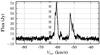 |
Fig. 7 Maser Cep-A: |


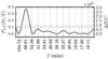 |
Fig. 8 Generalized Lomb-Scargle periodogram for maser Cep-A: |


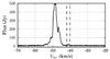 |
Fig. 9 Maser W 3(2): RA = 2h21m53s, Dec = 61°52′20′′, Dist ~2000 pc (RT-22, September 03, 2009, Puschino RAO RAS). |
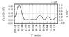 |
Fig. 10 Generalized Lomb-Scargle periodogram for maser W 3(2): RA = 2h21m53s, Dec = 61°52′20′′ (RT-22, September 03, 2009, Puschino RAO RAS). |
Acknowledgments
The authors express their gratitude to the anonymous referee for the valuable criticism and remarks.
References
- Goedhart, S., Maswanganye, J., Gaylard, M., & van der Walt, D. 2014, MNRAS, 437, 1808 [NASA ADS] [CrossRef] [Google Scholar]
- Imai, H., Deguchi, S., & Sasao, T. 2002, ApJ, 567, 971 [NASA ADS] [CrossRef] [Google Scholar]
- Ivezić, Ž., Connolly, A., Vanderplas, J., et al. 2014, Statistics, Data Mining and Machine Learning in Astronomy (Princeton, NJ: Princeton Univ. Press) [Google Scholar]
- Lekht, E., & Munitsyn, V. 2010, Astron. Rep., 54, 151 [NASA ADS] [CrossRef] [Google Scholar]
- Levenberg, K. 1944, Quart. Appl. Math., 2, 164 [Google Scholar]
- Lomb, N. 1976, Ap&SS, 39, 447 [NASA ADS] [CrossRef] [Google Scholar]
- Marquardt, D. 1963, J. Soc. Indust. Appl. Math., 11, 431 [Google Scholar]
- Reid, M., & Morgan, J. 1981, ARA&A, 19, 231 [NASA ADS] [CrossRef] [Google Scholar]
- Samodurov, V., Volvach, A., Siparov, S., et al. 2010, AIP Conf. Proc., 1206, 346 [NASA ADS] [CrossRef] [Google Scholar]
- Scargle, J. 1982, ApJ, 236, 835 [NASA ADS] [CrossRef] [Google Scholar]
- Siparov, S., & Samodurov, V. 2009, Comp. Optics, 30, 79 [Google Scholar]
- Vitiazev, V. 2001, Analysis of uneven time series (St.-Petersburg, RF: SPb Univ. Press) [in Russian] [Google Scholar]
- Zechmeister, M., & Kurster, M. 2009, A&A, 496, 577 [NASA ADS] [CrossRef] [EDP Sciences] [Google Scholar]
All Figures
|
Fig. 1 Maser W3(OH): RA = 2h23m18s, Dec = 61°38′58′′, Dist ~2000 pc (RT-22, June 30, 2009, Puschino RAO RAS). |
| In the text | |
|
Fig. 2 Time dependence of the selected detail shown in Fig. 1. |
| In the text | |
|
Fig. 3 Preliminary FFT analysis of the dependence on time of the power spectrum density for the feature marked in Fig. 1. |
| In the text | |
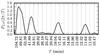 |
Fig. 4 Lomb-Scargle periodogram for the power spectrum density for the feature marked in Fig. 1. |
| In the text | |
|
Fig. 5 Generalized Lomb-Scargle periodogram for the power spectrum density for the feature marked in Fig. 1; ΔBIC is the Bayesian information criterion; the dotted lines show the 1% and 5% significance levels. |
| In the text | |
|
Fig. 6 Generalized Lomb-Scargle periodogram for the power spectrum density for maser W3(OH): RA = 2h23m18s, Dec = 61°38′58′′ (RT-22, June 26, 2009, Puschino RAO RAS). |
| In the text | |
|
Fig. 7 Maser Cep-A: |
| In the text | |
|
Fig. 8 Generalized Lomb-Scargle periodogram for maser Cep-A: |
| In the text | |
|
Fig. 9 Maser W 3(2): RA = 2h21m53s, Dec = 61°52′20′′, Dist ~2000 pc (RT-22, September 03, 2009, Puschino RAO RAS). |
| In the text | |
|
Fig. 10 Generalized Lomb-Scargle periodogram for maser W 3(2): RA = 2h21m53s, Dec = 61°52′20′′ (RT-22, September 03, 2009, Puschino RAO RAS). |
| In the text | |
Current usage metrics show cumulative count of Article Views (full-text article views including HTML views, PDF and ePub downloads, according to the available data) and Abstracts Views on Vision4Press platform.
Data correspond to usage on the plateform after 2015. The current usage metrics is available 48-96 hours after online publication and is updated daily on week days.
Initial download of the metrics may take a while.