| Issue |
A&A
Volume 574, February 2015
|
|
|---|---|---|
| Article Number | A57 | |
| Number of page(s) | 5 | |
| Section | Stellar structure and evolution | |
| DOI | https://doi.org/10.1051/0004-6361/201424511 | |
| Published online | 23 January 2015 | |
The CoRoT chemical peculiar target star HD 49310⋆
1
Department of Theoretical Physics and AstrophysicsMasaryk
University,
Kotlářská 2,
61 137
Brno,
Czech Republic
e-mail:
This email address is being protected from spambots. You need JavaScript enabled to view it.
2
Astrophysikalisches Institut Potsdam (AIP),
An der Sternwarte 16,
14482
Potsdam,
Germany
3
Department of Astrophysics, University of Vienna,
Türkenschanzstr. 17,
1180
Vienna,
Austria
Received: 2 July 2014
Accepted: 25 November 2014
Abstract
Context. The magnetic chemically peculiar (CP) stars of the upper main sequence are well-suited laboratories for investigating the influence of local magnetic fields on the stellar surface because they produce inhomogeneities (spots) that can be investigated in detail as the star rotates.
Aims. We studied the inhomogeneous surface structure of the CP2 star HD 49310 based on high-quality CoRoT photometry obtained during 25 days. The data have nearly no gaps. This analysis is similar to a spectroscopic Doppler-imaging analysis, but it is not a tomographic method.
Methods. We performed detailed light-curve fitting in terms of stationary circular bright spots. Furthermore, we derived astrophysical parameters with which we located HD 49310 within the Hertzsprung-Russell diagram. We also investigated the possible connection of this star to the nearby young open cluster NGC 2264.
Results. With a Bayesian technique, we produced a surface map that shows six bright spots. After removing some artefacts, the residuals of the observed and synthetic photometric data are ± 0.123 mmag. The rotational period of the star is P = 1.91909 ± 0.00001 days. Our photometric observations therefore cover about 13 full rotational cycles. Three spots are very large with diameters of ≃ 40deg. The spots are brighter by 40% than the unperturbed stellar photosphere.
Conclusions. HD 49310 is a classical silicon (CP2) star with a mass of about 3 M⊙. It is not a member of NGC 2264. Our analysis shows the potential of using high-quality photometric data to analyse the surface structure of CP stars. A comprehensive analysis of similar archival data, preferrably from space missions, would contribute significantly to our understanding of surface phenomena of CP stars and their temporal evolution.
Key words: stars: chemically peculiar / stars: individual: HD 49310
The CoRoT space mission was developed and is operated by the French space agency CNES, with participation of ESA’s RSSD and Science Programmes, Austria, Belgium, Brazil, Germany, and Spain.
© ESO, 2015
1. Introduction
About 10% of the upper main sequence stars between early-B and late-F type are characterised by remarkably rich line spectra. Compared to the Sun, overabundances are often inferred for some iron peak and rare-earth elements, while some other chemical elements, for example, scandium, might be underabundant. The chemically peculiar (CP) stars are commonly subdivided into four groups according to Preston (1974): metallic line stars (CP1), magnetic Ap stars (CP2), HgMn stars (CP3), and He-weak stars (CP4). CP2 and CP4 stars exhibit organised magnetic fields with a typical strength of a few hundred up to a few tens of thousand of Gauss. Chemical peculiarities are due to the diffusion of the chemical elements, which result from the competition between radiative pressure and gravitational settling. In magnetic stars this is guided by the magnetic field, possibly in combination with the influence of a weak magnetically directed wind (e.g., Babel 1992).
Many CP2 and CP4 stars exhibit photometric variability as a result of rotational modulation. While brightness variations of solar-type stars arise from activity induced by dynamo action inside the star and the related temperature spots, the physical nature of photometric variations of CP stars is directly connected with the radiative flux redistribution caused by enhanced or deficient opacity in abundance spots relative to the rest of the stellar surface (Krtička et al. 2012). Hence, as a star rotates, the observer sees different stellar regions that emit a different amount of radiative flux, which produces the characteristic index variability in phase-resolved photometry. Because the magnetic field of CP stars is inclined at a certain angle to their rotation axis (oblique-rotator model, Stibbs 1950), the observed variations are coupled with the apparent magnetic field as the star rotates.
Later on, this theory led to the development (Deutsch 1970) of the Doppler and magnetic Doppler-imaging technique, based on which these surface inhomogeneities can be mapped. However, this technique relies on high-resolution spectra with a high signal-to-noise ratio. Getting the corresponding data and subsequently analysing them for such a detailed investigation is very time-consuming. Up to now, only about fifteen CP stars were investigated in detail with these spectroscopic techniques (Nesvacil et al. 2012).
Large-scale photometric surveys with high data cadence that cover a long time-base, such as CoRoT, Kepler, and MOST, carry a significant potential for photometric surface mapping of a large sample of spotted stars.
We present a detailed analysis of the photometric light curve of HD 49310, a classical CP2 star, from the CoRoT (Convection, Rotation and planetary Transits) archive. CoRoT was a space mission that focused on high-precision photometry from space, taking advantage of observing given targets continuously for up to half a year (Baglin et al. 2006).
2. Target star and observations
HD 49310 (BD +10 1270, V = 9.13 mag) is situated in the Monoceros star-forming region where the young open cluster NGC 2264 is also located. It was classified as Ap Si by Bidelman & MacConnell (1973).
We compiled the Geneva photometry from the General Catalogue of Photometric data (Mermilliod et al. 1997); the Strömgren uvbyβ photometry was taken from Masana et al. (1998). We calculated the peculiarity index p (Masana et al. 1998) to be 1.73, which is higher than the threshold for normal-type stars of 1.50. In addition, we derived the peculiar indices of the Geneva system: Δ(V1 − G) = +29 mmag and Z = −40 mmag. These values are also compatible with the spectral classification as an Ap star (Paunzen et al. 2005).
The effective temperature was derived on the basis of photometric calibrations given by Netopil et al. (2008). This calibration is best suited because it is specifically tuned for the different types of CP stars. The final Teff = 11 500 ± 500 K is the average Teff, and its standard deviation was obtained by calibrating the different photometric systems and colours. From the same paper we took the bolometric correction to derive the luminosity of log L/L⊙ = 2.03 ± 0.12 dex. The latter corresponds to a log g = 4.05 ± 0.10 dex. From these values and by applying the full error propagation (Sódor et al. 2009), we derive log R/R⊙ = 0.42 ± 0.06 dex.
As a next step, we investigated whether HD 49310 is a member of the young open cluster NGC 2264 (age younger than 5 Myr, distance of about 760 pc from the Sun, Cody et al. 2014) as suggested by Karlsson (1972). If this is true, HD 49310 is still in its pre-main-sequence phase. From these calibrations, we conclude that the star is not reddened. With the apparent and absolute magnitude, we calculated a distance of about 600 pc. Grenier et al. (1999) published a radial velocity of +10.1 ± 1.9 km s-1 for HD 49310, while the cluster mean of NGC 2264 is +22 km s-1 (Fürész et al. 2006). Furthermore, we searched for an IR-excess, as is typical for pre-main-sequence stars of this estimated mass (Costigan et al. 2014). The tool VO Sed Analyzer (VOSA, Bayo et al. 2008) was used for this purpose. The photometry of the Wide-Field Infrared Survey Explorer (WISE) in the infrared revealed no excess. Therefore, we conclude that HD 49310 is not associated with NGC 2264.
Figure 1 shows the Hertzsprung-Russell diagram for HD 49310 and the sample of well-established CP2 stars (with available parallaxes from the Hipparcos mission) from Netopil et al. (2008) together with lines of equal masses and radii calculated from the evolutionary grids of solar metallicity by Schaller et al. (1992). The location of HD 49310 is well within the area of the comparison sample. From the diagram, we conclude that the mass range is of about 2.9 M⊙ to 3.3 M⊙ and the radius of about 2.3 R⊙ to 3.2 R⊙. It spent between 20% to 70% of its main-sequence lifetime, which corresponds to an age between 80 Myr and 280 Myr.
HD 49310 was observed by the CoRoT satellite from March 5 until March 31, 2008. The time span of 25.3 days covers 13.2 stellar rotational cycles. The light curve (see Fig. 2) of HD 49310 exhibits a periodic behaviour with an overall variation in brightness of 0.017 mag.
To save computational time, the 60 553 original data points (with a time resolution of about 30 s) were combined into bins of maximal width of 0.01 days (which is roughly one-seventh of the orbital period of CoRoT). Within a bin, the time difference between adjacent points must not exceed 0.0004 days. Each of the 2417 final data points was assigned a weight according to the number of contributing original data points within a bin.
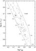 |
Fig. 1 Hertzsprung-Russell diagram for HD 49310 (filled circle) and the sample of well-established CP2 stars (open circles) from Netopil et al. (2008). The full lines represent the zero- and terminal-age main-sequence from the evolutionary grids by Schaller et al. (1992) for solar metallicity. The stellar mass and radius, relative to each track, are indicated in the plot in solar units. |
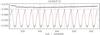 |
Fig. 2 2417 data points fitted by a six-spot model (red line). In the upper part the residuals (arbitrary offset) are shown. Jumps and linear trends are accounted for automatically by using a likelihood function that integrates over all possible magnitude offsets and trends. This was made individually for each part of the light curve. Without the systematics the contingent part of the residuals is ± 0.123 mmag. |
3. Bayesian spot modelling
The original CoRoT data for HD 49310 include gaps, small jumps, and spurious trends. These trends and discontinuities are probably artefacts resulting from drifting detector sensitivities, cosmic-ray hits of the CCD, and other instrumental effects of CoRoT (Mazeh et al. 2009). Before the binning, the light curve shown in Fig. 2 was divided into thirteen parts according to the jumps and trend changes occurring between adjacent parts. The likelihood function is vital for any parameter estimation. This is here the product of thirteen contributions determined for the thirteen individual parts. The likelihood for each part was constructed as follows: it was assumed that the residuals (“errors” in the magnitude domain), that is, the deviations between observation and theoretical model, hence measurement errors augmented by systematic (model) errors, are Gaussian-distributed with unknown variance. Because the 2417 data points were assigned different weights, we furthermore assumed that a data-point variance is given by some common variance divided by the individual weight. The latter is simply the number of original data points within a bin. To overcome this common but nevertheless unknown variance, the Gaussian likelihood function was integrated over this unknown variance by applying Jeffreys’ prior (Jeffreys 1961). In this case, the prior is the reciprocal of the variance. This error-integrated likelihood was then integrated over all possible magnitude offsets and even all possible linear trends. These three integrations were made analytically. The fact that the error variance, magnitude offset, and trend can be dismissed is a comfortable feature of this type of data analysis because it reduces the number of free parameters and enhances robustness. The disadvantage is that these parameters of no immediate interest remain undetermined. When overplotting the corrected data on a model for a smooth presentation (Fig. 2), offsets and trends have to be applied to minimize the mean squared distance between the data and the model.
The resulting combined likelihood is a function of the data alone, given a set of parameter values.
The following parameters were estimated: the stellar inclination, cos(i), the rotation period, log (P), the common spot brightness, κ, in units of stellar surface brightness, and the central longitude, λ, latitude, sin(β), and area, log (A), for each circular spot. The longitude increases in the direction of stellar rotation. The zero point is the central meridian facing the observer at the beginning of the time series. The area is in units of the stellar cross section.
Each parameter is presented in such a way that its prior distribution is flat. The logarithms, for instance, ensure that the results in the case of non-dimensionless parameters are independent of any preferences, meaning that it does not matter whether one prefers period or frequency, spot area, or radius. As all parameter priors are flat, the likelihood mountain across the parameter space reflects the desired posterior density distribution.
To mitigate the effects of correlations between the parameters of interest, we performed a Markov chain Monte Carlo (MCMC) exploration of parameter space in a formally more suited transformed space. Each parameter in the transformed space was represented as a linear combination of all the original parameters. The de-correlating transformation was based on singular value decomposition (cf. Press et al. 2007). No compression was applied during the back-transformation into the original parameter space. As a result of correlations among the parameters, there are always fewer degrees of freedom of the parameter estimation problem than there are free parameters – in our case about a quarter of the number of free parameters.
The two coefficients of the quadratic limb-darkening relation were taken from the Claret & Bloemen (2011) tables, assuming an effective temperature of 11 500 K, a surface gravity of 4.05 dex, and solar metallicity. With respect to limb darkening, no difference was made between unperturbed photosphere and spots.
Theoretical light curves were computed using Dorren’s analytical formulae (Dorren 1987), but generalized for quadratic limb darkening.
As was shown previously (Lüftinger et al. 2010), Si, which probably is the main element responsible for the light-curve variations of HD 49310, causes bright spots instead of dark ones (see e.g. also Mikulášek et al. 2008; Krtička et al. 2012).
Moreover, we searched for stationary oscillations that are superimposed to the spot-induced light variation. We only searched within two restricted frequency regions: around the orbital frequency of the CoRoT satellite and around one day.
Finally, a solution with six bright spots yielded the best Bayesian fit to the data. In total, a set of 44 free parameters was estimated (see Table 1).
Stellar and star-spot parameters for the six-spot solution and – for comparison – a four-spot solution.
4. Results of photometric spot modelling
In our case of six spots, the result of a Bayesian parameter estimation is the posterior probability distribution across a 44-dimensional space. By marginalization, that is, by neglecting the information on correlations, this yields 44 marginal distributions. Each marginal distribution reveals the probability distribution of a parameter, irrespective of the values of all the other parameters. It can be comfortably summarized by its expectation value and usual credibility interval(s). It is an advantage of the Bayesian approach that parameter averages such as median, expectation, and modal value as well as the credibility intervals are deduced from the measured data alone. It is not necessary to rely on artificial or reshuffled data.
Table 1 lists the expectation values and the 68.3% (i.e. ±one-σ) credibility intervals for all spot-modelling parameters. If necessary, the probability distributions were transformed accordingly. The probability distribution for the stellar rotational period, P, for instance, was derived from the marginal distribution of log e(P). The expectation for P, ⟨ P ⟩, therefore differs somewhat from exp( ⟨ log e(P) ⟩ ), with ⟨ log e(P) ⟩ being the expectation of log e(P).
For comparison, the results for a four-spot model are listed as well. The surface mapping proves to be rather stable, meaning that the main features are already covered by four spots. As expected, the spot latitudes are the least constrained parameters.
The Bayesian information criterion (BIC1, Schwarz 1978) indicates that the six-spot model is to be preferred. The gain in goodness-of-fit by considering six spots more than compensates for the loss of credibility due to the larger number of free parameters. Whether including a seventh spot would justify the numerical effort remains undecided, as this investigation would require excessive computing power.
At first glance, the smallness of the one-σ errors in Table 1 seems unrealistic, but this is a well-known feature of any Bayesian analysis. Errors resulting from the posterior probability distribution over the parameter space only measure the freedom of movement in an idealized model. Only in the unlikely case that the model is able to match nature perfectly, that is, when all assumptions are completely fulfilled in all detail, the errors would describe the uncertainty of our knowledge about real stellar spots. There is certainly more information in the CoRoT high-precision data than we can summarize in terms of six persistent circular spots with uniform surface brightness. Nevertheless, our six-spot model describes the essential features of the star best. As computational cost is a problem, assuming circularity of the spots is necessary because otherwise the computational demand in the absence of analytical formulae is prohibitive.
The rotation period can be estimated accurately to within ± 2 ppm thanks to the nearly 13.2 rotations covered by high-precision CoRoT data and thanks to an elaborate spot model.
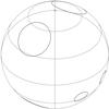 |
Fig. 3 Five of the six spots at JD 2 454 531.48. |
Three HARPS spectra of HD 49310 are available in the ESO archive2. Although the individual spectra are very noisy, it is possible to derive the projected rotational velocity from the combined spectrum to υsini = 70 ± 2 km s-1, which excludes a rotational period twice as long. This is very important additional information because several Ap stars show double-wave photometric variations (Maitzen et al. 1978), leading to an incorrect rotational period. Using the values from Table 1, we derive log R/R⊙ = 0.51 ± 0.03 dex. Within the errors, the estimated stellar radius agrees with the radius derived from photometry (see Sect. 2).
The second spot has the same size as the first and is located at the opposite longitude (see Fig. 3).
The sixth spot is the largest but admittedly barely visible, which explains why its location and radius are less constrained than the corresponding parameters of the other five spots.
In addition to the stellar rotational period of 1.9191 days, we found three very likely non-stellar oscillations including overtones: the CoRoT orbital period of  ±
± , the “sidereal” day
  , and the more “common” day
  ±
± . The signal with the CoRoT orbital period has an amplitude of 61±1 ppm, and its higher harmonics are 17±1 ppm, 12±1.5 ppm, and 13±1.5 ppm, respectively. The strongest variation related to a day is the half “sidereal” day with an amplitude of 27±2 ppm, but perhaps there are more than two periods close to one day.
In view of the accuracy of the photometric data, it is interesting to search for differential rotation. Describing the latitudinal dependence of the angular velocity by a sin2-law, one needs another free parameter in addition to the equatorial period. The gain in fit accuracy is marginal. Moreover, the outcome is inconclusive because it is impossible to disctinguish solar-like differential rotation against anti-solar rotation. The lapping time exceeds 200 years in both cases. Hence, there is no reason to reject the hypothesis of rigid rotation.
5. Conclusion and outlook
We analysed the high-quality CoRoT light curve of the CP2 star HD 49310. With available very precise long-term and continuous photometric data, mainly based on space missions, an alternative to the classical Doppler imaging technique is possible: the photometric modelling of star spots, as presented in this paper. Lüftinger et al. (2010) investigated in detail spectroscopic and photometric time-series for the CP2 star HD 50773. They used an extensive set of ground-based spectropolarimetric data for Doppler and magnetic Doppler imaging together with photometric CoRoT data and found an excellent correlation of the surface maps in terms of spot location and size from the photometric and spectroscopic data.
We fitted a model with six bright spots to the CoRoT data of HD 49310, which is a silicon star with about 3 M⊙ and an age between 80 Myr and 280 Myr. The three largest spots are, as expected, near the poles of the star.
Furthermore, we propose to systematically analyse the light curves of the Kepler space mission (Chaplin 2011) of bona fide magnetic CP stars which has not been attempted so far, to our knowledge. This would help understanding the characteristics of stellar spots for objects at the upper main sequence in connection with a local magnetic field.
We rely on this criterion because we are unable to compute evidence by integrating the posterior distribution over the whole parameter space in a strict Bayesian manner to rank hypotheses that differ in the number of spots. Shortage of computing power forces us to exploit the accessible BIC to choose the trade-off between simplicity-of-model and goodness-of-fit.
Acknowledgments
This project is financed by the SoMoPro II programme (3SGA5916). The research leading to these results has acquired a financial grant from the People Programme (Marie Curie action) of the Seventh Framework Programme of EU according to the REA Grant Agreement No. 291782. The research is furthermore co-financed by the South-Moravian Region. It was also supported by grants GP14-26115P, 7AMB14AT015, the financial contributions of the Austrian Agency for International Cooperation in Education and Research (BG-03/2013 and CZ-09/2014), and the Austrian Research Fund via the project FWF P22691-N16. This research has made use of the WEBDA database, operated at the Department of Theoretical Physics and Astrophysics of the Masaryk University. Based on observations made with ESO Telescopes at the La Silla Observatory under programme ID 182.D-0356. The MCMC computations have been performed at the AIP. This work reflects only the author’s views and the European Union is not liable for any use that may be made of the information contained therein.
References
- Babel, J. 1992, A&A, 258, 449 [NASA ADS] [Google Scholar]
- Baglin, A., Michel, E., Auvergne, M., et al. 2006, in ESA SP, 1306, 3950 [Google Scholar]
- Bayo, A., Rodrigo, C., Barrado y Navascues, D., et al. 2008, A&A, 492, 277 [NASA ADS] [CrossRef] [EDP Sciences] [Google Scholar]
- Bidelman, W. P., & MacConnell, D. J. 1973, AJ, 78, 687 [NASA ADS] [CrossRef] [Google Scholar]
- Chaplin, W. J., Kjeldsen, H., Christensen-Dalsgaard, J., et al. 2011, Science, 332, 213 [NASA ADS] [CrossRef] [PubMed] [Google Scholar]
- Claret, A., & Bloemen, S. 2011, A&A, 529, A75 [NASA ADS] [CrossRef] [EDP Sciences] [Google Scholar]
- Cody, A. M., Stauffer, J., Baglin, A., et al. 2014, AJ, 147, 82 [NASA ADS] [CrossRef] [Google Scholar]
- Costigan, G., Vink, J. S., Scholz, A., Ray, T., & Testi, L. 2014, MNRAS, 440, 3444 [NASA ADS] [CrossRef] [Google Scholar]
- Deutsch, A. J. 1970, ApJ, 159, 985 [NASA ADS] [CrossRef] [Google Scholar]
- Dorren, J. D. 1987, ApJ, 320, 756 [NASA ADS] [CrossRef] [Google Scholar]
- Fürész, G., Hartmann, L. W., Szentgyorgyi, A. H., et al. 2006, ApJ, 648, 1090 [NASA ADS] [CrossRef] [Google Scholar]
- Grenier, S., Baylac, M.-O., Rolland, L., et al. 1999, A&AS, 137, 451 [NASA ADS] [CrossRef] [EDP Sciences] [Google Scholar]
- Jeffreys, H. 1961, Theory of Probability, 3rd edn. (Oxford: Oxford Univ. Press) [Google Scholar]
- Karlsson, B. 1972, A&AS, 7, 35 [NASA ADS] [Google Scholar]
- Krtička, J., Mikulášek, Z., Lüftinger, T., et al. 2012, A&A, 537, A14 [NASA ADS] [CrossRef] [EDP Sciences] [Google Scholar]
- Lüftinger, T., Fröhlich, H.-E., Weiss, W. W., et al. 2010, A&A, 509, A43 [NASA ADS] [CrossRef] [EDP Sciences] [Google Scholar]
- Maitzen, H. M., Albrecht, R., & Heck, A. 1978, A&A, 62, 199 [NASA ADS] [Google Scholar]
- Masana, E., Jordi, C., Maitzen, H. M., & Torra, J. 1998, A&AS, 128, 265 [NASA ADS] [CrossRef] [EDP Sciences] [Google Scholar]
- Mazeh, T., Guterman, P., Aigrain, S., et al. 2009, A&A, 506, 431 [NASA ADS] [CrossRef] [EDP Sciences] [Google Scholar]
- Mermilliod, J.-C., Mermilliod, M., & Hauck, B. 1997, A&AS, 124, 349 [NASA ADS] [CrossRef] [EDP Sciences] [Google Scholar]
- Mikulášek, Z., Krtička, J., Henry, G. W., et al. 2008, A&A, 485, 585 [NASA ADS] [CrossRef] [EDP Sciences] [Google Scholar]
- Nesvacil, N., Lüftinger, T., Shulyak, D., et al. 2012, A&A, 537, A151 [NASA ADS] [CrossRef] [EDP Sciences] [Google Scholar]
- Netopil, M., Paunzen, E., Maitzen, H. M., North, P., & Hubrig, S. 2008, A&A, 491, 545 [NASA ADS] [CrossRef] [EDP Sciences] [Google Scholar]
- Paunzen, E., Stütz, Ch., & Maitzen, H. M. 2005, A&A, 441, 631 [NASA ADS] [CrossRef] [EDP Sciences] [Google Scholar]
- Press, W. H., Teukolsky, S. A., Vetterling, W. T., & Flannery, B. P. 2007, Numerical Recipes, 3rd edn. (Cambridge: Cambridge Univ. Press) [Google Scholar]
- Preston, G. W. 1974, ARA&A, 12, 257 [NASA ADS] [CrossRef] [MathSciNet] [Google Scholar]
- Schaller, G., Schaerer, D., Meynet, G., & Maeder, A. 1992, A&AS, 96, 269 [Google Scholar]
- Schwarz, G. 1978, Ann. Stats., 6, 461 [Google Scholar]
- Sódor, Á., Jurcsik, J., & Szeidl, B. 2009, MNRAS, 394, 261 [NASA ADS] [CrossRef] [Google Scholar]
- Stibbs, D. W. N. 1950, MNRAS, 110, 395 [NASA ADS] [CrossRef] [Google Scholar]
All Tables
Stellar and star-spot parameters for the six-spot solution and – for comparison – a four-spot solution.
All Figures
|
Fig. 1 Hertzsprung-Russell diagram for HD 49310 (filled circle) and the sample of well-established CP2 stars (open circles) from Netopil et al. (2008). The full lines represent the zero- and terminal-age main-sequence from the evolutionary grids by Schaller et al. (1992) for solar metallicity. The stellar mass and radius, relative to each track, are indicated in the plot in solar units. |
| In the text | |
|
Fig. 2 2417 data points fitted by a six-spot model (red line). In the upper part the residuals (arbitrary offset) are shown. Jumps and linear trends are accounted for automatically by using a likelihood function that integrates over all possible magnitude offsets and trends. This was made individually for each part of the light curve. Without the systematics the contingent part of the residuals is ± 0.123 mmag. |
| In the text | |
|
Fig. 3 Five of the six spots at JD 2 454 531.48. |
| In the text | |
Current usage metrics show cumulative count of Article Views (full-text article views including HTML views, PDF and ePub downloads, according to the available data) and Abstracts Views on Vision4Press platform.
Data correspond to usage on the plateform after 2015. The current usage metrics is available 48-96 hours after online publication and is updated daily on week days.
Initial download of the metrics may take a while.