| Issue |
A&A
Volume 573, January 2015
|
|
|---|---|---|
| Article Number | A20 | |
| Number of page(s) | 7 | |
| Section | Stellar structure and evolution | |
| DOI | https://doi.org/10.1051/0004-6361/201424867 | |
| Published online | 09 December 2014 | |
Magnetorotational instability in decretion disks of critically rotating stars and the outer structure of Be and Be/X-ray disks
Department of Theoretical Physics and AstrophysicsMasaryk
University,
Kotlářská 2,
611 37
Brno,
Czech Republic
e-mail:
This email address is being protected from spambots. You need JavaScript enabled to view it.
Received: 27 August 2014
Accepted: 17 October 2014
Abstract
Context. Evolutionary models of fast-rotating stars show that the stellar rotational velocity may approach the critical speed. Critically rotating stars cannot spin up more, therefore they lose their excess angular momentum through an equatorial outflowing disk. The radial extension of such disks is unknown, partly because we lack information about the radial variations of the viscosity.
Aims. We study the magnetorotational instability, which is considered to be the origin of anomalous viscosity in outflowing disks.
Methods. We used analytic calculations to study the stability of outflowing disks submerged in the magnetic field.
Results. The magnetorotational instability develops close to the star if the plasma parameter is large enough. At large radii the instability disappears in the region where the disk orbital velocity is roughly equal to the sound speed.
Conclusions. The magnetorotational instability is a plausible source of anomalous viscosity in outflowing disks. This is also true in the region where the disk radial velocity approaches the sound speed. The disk sonic radius can therefore be roughly considered as an effective outer disk radius, although disk material may escape from the star to the insterstellar medium. The radial profile of the angular momentum-loss rate already flattens there, consequently, the disk mass-loss rate can be calculated with the sonic radius as the effective disk outer radius. We discuss a possible observation determination of the outer disk radius by using Be and Be/X-ray binaries.
Key words: stars: mass-loss / stars: evolution / stars: rotation / hydrodynamics / magnetohydrodynamics (MHD)
© ESO, 2014
1. Introduction
Accretion is one of the most ubiquitous processes in astrophysics and occurs in different environments on various length scales. The crucial problem of accretion is that the accreting matter has to lose its angular momentum on Keplerian orbits while moving towards the centre of gravity. If the corresponding angular momentum transfer would have to rely on the molecular viscosity alone, the time of accretion would be prohibitively long. Consequently, some type of anomalous viscosity has to be present in disks that allows the accretion to proceed in time compatible with observational constraints. Magnetorotational instability (MRI, Balbus & Hawley 1991) is considered to be the main source of anomalous viscosity in such disks.
In contrast, decretion disks are connected with stellar mass-loss, but their presence stems from the same principle as the existence of the accretion disk, that is, the need for angular momentum transport. Evolutionary models of fast-rotating stars show that the stellar rotational velocity may approach the critical velocity (Meynet et al. 2006; Ekström et al. 2008), above which no stellar spin-up is possible. The further evolution of a critically rotating star may require loss of angular momentum, which is achieved through an outflowing decretion disk (Krtička et al. 2011). The disk may extend to several hundred stellar radii (Kurfürst et al. 2014) or even more. The angular momentum transport in the disk requires some type of anomalous viscosity, which is presumably connected with MRI.
Decretion disks are typically connected with Be and B[e] star disks (Lee et al. 1991; Okazaki 2001). Classical Be stars are non-supergiant B stars, whose hydrogen lines have (or had in the past) an emission component that can be explained by an equatorial disk (see Rivinius et al. 2013, for a review). The observational evidence supports the picture that the material of the disk comes from the star, and therefore the disks are called decretion disks. The mechanism that transports the stellar material into the disk is unclear at present. However, it is generally believed that once the material appears in the disk, it has a Keplerian rotation and is transported away from the star by the same anomalous viscosity that operates in accretion disks.
However, it is unclear whether the MRI can operate in decretion disks of Be stars. From an observational and theoretical point of view, the Be star disks can extend to the distances of at least hundreds of stellar radii, and it is unclear whether the angular momentum transport in the distant regions is the same as close to the star. Therefore, we provide here an analytic study of MRI in the decretion disks of Be stars, which will be accompanied by a detailed magnetohydrodynamical modelling in a future paper.
2. Basic physics of MRI
Magnetorotational instability can exist even in very weakly magnetized disks. If there is a radial displacement in such disks, the magnetic stresses may win and push the material back towards its original position. These displacements do not cause any instability. The displaced material is kept on corotation with respect to its original position. If the centrifugal force acting on the displaced material is higher than the force due to magnetic stresses, the material accelerates in the direction of the original displacement, leading to an instability.
The behaviour of the displaced particle in the disk submerged in the magnetic field with a zero radial component can be described by a dispersion relation (Balbus & Hawley 1991) 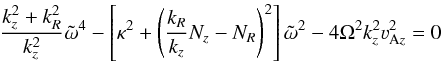 (1)in the cylindrical coordinates (R,φ,z), where
  (2)the square of the epicyclic frequency is
 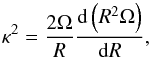 (3)the pieces of the Brunt-Väisälä frequency
  are
are ![Mathematical equation: % subequation 711 0 \begin{eqnarray} \label{jesenius} N_R^2&=&-\frac{3}{5\rho}\frac{\partial P}{\partial R} \frac{\partial\ln P\rho^{-5/3}}{\partial R}, \\[2mm] N_z^2&=&-\frac{3}{5\rho}\frac{\partial P}{\partial z} \frac{\partial\ln P\rho^{-5/3}}{\partial z}, \end{eqnarray}](/articles/aa/full_html/2015/01/aa24867-14/aa24867-14-eq6.png) Ω is the angular velocity, kz and kR are vertical and radial wavenumbers, ω is the angular frequency, and the square of the vertical Alfvén velocity is
Ω is the angular velocity, kz and kR are vertical and radial wavenumbers, ω is the angular frequency, and the square of the vertical Alfvén velocity is  (5)where Bz is the vertical component of the magnetic field and ρ is the density. The instability occurs in the disks with radially decreasing angular velocity,
  (6)In such disks the dispersion relation Eq. (1)leads to instability (ω2< 0) for vertical wavenumbers kz<kz,max with
 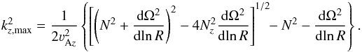 (7)This instability is thought to be the source of anomalous viscosity in accretion disks.
3. Stationary-disk model
As a starting point of our instability study we assumed an outflowing disk transporting an excess angular momentum from a critically rotating star (Krtička et al. 2011) with equatorial radius  (here R∗ is the stellar polar radius). The stationary-disk solution is derived from the equation of continuity, and equations of motion in radial and azimuthal directions. The static equations provide a radial dependence of the integrated disk density Σ, and radial νR and azimuthal νφ components of the velocity. For a simplicity, we assumed an isothermal disk with
  , which roughly corresponds to the NLTE models (Millar & Marlborough 1998; Carciofi & Bjorkman 2008).
The stellar parameters selected for the modelling correspond to the main-sequence B2–B3 star with an effective temperature Teff = 20 000 K, mass M = 6.60 M⊙, and radius R∗ = 3.71 R⊙ (Harmanec 1988). We also calculated additional models for main-sequence stars with different effective temperatures Teff = 30 000 K and Teff = 14 000 K and with radially decreasing disk temperature T = T0(Req/R)p with p = 0.1 and p = 0.2. The results of our models show that the properties of the disk model and our results in general do not significantly depend on the particular choice of the disk and stellar parameters. Consequently, below we mainly discuss a model with Teff = 20 000 K.
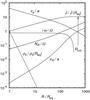 |
Fig. 1 Dependence of the radial and azimuthal velocities (in units of sound speed a), the midplane disk density ρ0 (relative to its value at R = Req), the angular momentum-loss rate in units of equator release angular momentum-loss rate |

In Fig. 1 we provide the radial dependences of selected variables. The radial disk velocity νR increases linearly with radius close to the star. In the same region the azimuthal velocity follows the Keplerian rotation νφ ~ R− 1 / 2. The midplane disk density ρ0 strongly decreases with radius because of disk acceleration, flaring, and geometrical reasons in total as ρ0 ~ R-3.5. The angular momentum loss  increases linearly with radius close to the star and is highest close to the critical radius Rcrit, where the radial velocity reaches the sound speed, νR = a (Okazaki 2001; Krtička et al. 2011).
4. MRI close to the star
The condition of the decreasing angular velocity Eq. (6)is fulfilled everywhere in the Be star disks. However, the disks are typically very thin close to the star. In a thin disk the lowest vertical wavenumber Eq. (7)could be too low for the development of the instability. Denoting a typical vertical disk thickness as 23 / 2H with  (8)where νK is the Keplerian rotation velocity at radius R and a is the sound speed, only the modes with wavelength lower than 23 / 2H can exist in the disk, giving the condition for the lowest wavelength leading to instability as
 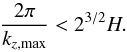 (9)Close to the star the Brunt-Väisälä frequency is negligible with respect to the angular velocity derivative in Eq. (7), yielding the wavenumbers leading to instability
 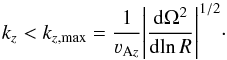 (10)Inserting the Alfvén speed Eq. (5)with the highest density corresponding to the midplane density ρ0, the conditions for the development of instability Eqs. (9)and (10)can be combined into a condition for the vertical magnetic field,
 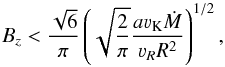 (11)where the disk mass-loss rate is Ṁ = (2π)3 / 2νRρ0RH (e.g., Krtička et al. 2011), and we assumed a Keplerian rotation Ω = νK/R. Physically, this means that the gas pressure has to dominate magnetic pressure and the plasma parameter β>π2/ 3 ≈ 3 (Balbus & Hawley 1991; Montani et al. 2013). For lower values of β only stable modes (kz>kz,max) can exist in the disk.
Equation (11)can be rewritten in scaled quantities as  (12)For a typical B star and disk parameters and νR ≈ 10-3a valid for viscosity parameter α ≈ 1 follows that the strongest vertical equatorial magnetic field that allows the instability to grow is of the order of tens of Gauss. In the presence of turbulence, the square of the external magnetic field
  can be amplified (Okuzumi & Ormel 2013; Fujii et al. 2014), implying the decrease of the strongest magnetic field Eq. (12)in the disk.
 |
Fig. 2 Zero-crossing root of the dispersion relation Eq. (1)as a function of radial and vertical wavenumbers at R = 1.01 Req for the model given in Fig. 1. The plane ω = 0 divides perturbations that are stable − ω2< 0 from that leading to an instability − ω2> 0. The red region denotes perturbations with a too large characteristic scale that can not be accommodated in the disk |

These conclusions are documented in Fig. 2, where we plot the zero-crossing root of the dispersion relation Eq. (1)in the midplane of the disk model described in Sect. 3 at R = 1.01 Req. This case leads to MRI, as for some wavenumbers the root becomes negative, − ω2> 0. The perturbations with  have a characteristic scale larger than the disk thickness 23 / 2H and do not exist in the disk. With increasing magnetic field intensity (or decreasing disk midplane density) the zone of the perturbations with a too large characteristic scale increases and fully encompasses the instability region − ω2> 0 for vertical fields stronger than that given in Eq. (11). For such strong magnetic fields the MRI ceases to exist close to the star.
In stars with a magnetic field stronger than that given by Eq. (12)the MRI does not operate in stationary conditions. Such stars may possibly accumulate the material close to their equator until the condition for the MRI development Eq. (10)is fulfilled. They may show episodic ejections of matter.
Close to the star, where the parts of the Brunt-Väisälä frequency NR and Nz are negligible, the square of the instability branch of MRI frequency has in the midplane from Eq. (1)an extremum for kR = 0 and  , yielding
  (13)Consequently, the ratio of the MRI instability growth rate to the angular frequency of the rotation ω/ Ω is constant close to the star. The numerical calculations in Fig. 1 show that Eq. (13)holds nearly up to the radius, where this root of the dispersion relation changes its sign. Moreover, Eq. (13)is also valid out of the midplane, in even slightly more radially extended region.
5. MRI at large distances from the star
From the radial dependence νR/a ~ R and νK ~ R− 1 / 2 the decrease of the limiting magnetic field Eq. (12)proportional to R-1.75 is slower than the decrease of magnetic field intensity of the dipolar field, which is proportional to R-3. This shows that the disks that develop MRI close to the star, are also unstable with respect to MRI at larger radii. Moreover, if the magnetic field does not lead to MRI close to the star, it may be weak enough for the development of MRI at larger radii.
However, despite this, the MRI may vanish at very large radii because of another effect. At the locations where the epicyclic frequency becomes too low,  the root of the dispersion relation Eq. (1) that was negative close to the star becomes positive and the instability vanishes. This can be seen for Keplerian rotation κ2 = Ω2, where Eq. (1) gives in the midplane where Nz = 0 (for concreteness for kR ≪ kz) for the approximation for the lower root of the dispersion relation
  (14)With increasing radii ω2 changes its sign from negative to positive at the point where from Eq. (14)
 (15)The latter identity follows from the definition of NR in Eq. (4a)assuming isothermal disks. For a radial density decrease proportional to ρ ~ R− n the limiting azimuthal velocity above which the instability does not develop is
  for considered disks. The disappearance of the MRI can be understood as a consequence of low orbital velocity. For orbital velocities lower than the sound speed the centrifugal acceleration becomes unimportant and the branch of the dispersion relation that for high rotational velocities corresponds to MRI changes to ordinary Alfvén waves.
This is demonstrated in Fig. 3, where we plot the root that may cross zero of the dispersion relation Eq. (1)in the midplane of the disk model described in Sect. 3 at R = 440 Req (where νφ = a). All roots of the dispersion relation are positive, ω2> 0 and the MRI does not occur here. We note that this occurs regardless the magnitude of the magnetic field. The same effect also appears above the midplane, but for slightly larger radii.
6. Time-dependent models with decreasing viscosity
We studied the consequences of MRI disappearance at large radii using time-dependent models with radially decreasing viscosity parameter. For these models we used the same set of basic hydrodynamic equations, the same disk conditions, and the same stellar parameters as in Sect. 3 for B2–B3 type star. We calculated the models of isothermal disk for a constant viscosity parameter α = α(Req) and with decreasing viscosity α = α(Req) [ (391 Req − R) / (390 Req) ] ≈ α(Req) [ 1 − R/ (390 Req) ], that is, up to the radius 390 Req the viscosity α parameter decreases relatively steeply and beyond this radius it is fixed at the constant value α = α(Req) / 390 (see the discussion in Sect. 9.3).
In the time-dependent models (unlike the stationary calculations) we can involve the full second-order Navier-Stokes prescription of the viscous torque. This provides physically more relevant distributions of rotational velocity (and consequently of the specific angular momentum-loss rate) even in very distant disk regions (for details see Kurfürst et al. 2014). The results of the models we obtain as a final stationary state of the converging time-dependent calculations.
Figure 4 compares the radial profiles of the relative disk midplane density ρ0/ρ0(Req) and of the scaled radial and azimuthal velocities νR/a and νφ/a (where a is the speed of sound) as well as of the scaled specific angular momentum-loss rate  (cf. Fig. 1 in Sect. 3) for the two cases of radial viscosity distribution. The profile of the relative midplane maximum MRI growth rate iω/ Ω is calculated following Eq. (1)where we involve the full prescription of the epicyclic frequency κ (see Eq. (3)) and the radial piece of Brunt-Väisälä frequency NR (Eq. (4a)).
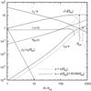 |
Fig. 4 Final stationary state of time-dependent disk models with constant and variable viscosity parameter α. We plot the same variables as in the stationary model in Fig. 1. In the constant-viscosity model (dashed line) the viscosity parameter α = α(Req), while in the decreasing-viscosity model (solid line) the parameter α = α(Req)[ (391 Req − R) / (390 Req) ] below R = 390 Req and α = α(Req) / 390 elsewhere. The inner boundary viscosity parameter α(Req) = 0.1. We consider the isothermal disk of the main-sequence B2–B3 type star (see Sect. 3). Arrows denote the locations of the critical points. |
The time-dependent calculations show that the decretion disks may spread to large radii despite the vanishing MRI instability. For a constant viscosity distribution the rotational velocity (and and the angular momentum-loss rate  ) begins to drop rapidly even below the sonic (critical) point distance. This can be avoided in the model with a decreasing viscosity coefficient (Kurfürst et al. 2014). Moreover, Eq. (13)is also valid for a decreasing viscosity in the Keplerian region, but the radius where the MRI instability vanishes (the root of the dispersion relation changes its sign) increases for a decreasing viscosity.
From our time-dependent models (see Kurfürst et al. 2014) it follows that the disks are developed to very far distances even for a radially decreasing viscosity parameter. The reason is likely the high radial velocity in the distant supersonic regions (even though the disk radial velocity in the distant regions is about one order of magnitude lower than for line-driven stellar winds). During the disk-developing phase we also recognize the wave with supersonic speed that propagates to these far distant disk regions; we assume that a similar transforming wave occurs and that its amplitude and velocity depend on physical conditions (the density distribution) in the stellar surroundings.
Our models also confirm the dependence of the sonic point distance and of the distance of the disk outer edge (i.e., the radius where the rotational velocity begins to rapidly decrease, see Fig. 4) on the parameterized viscosity and temperature profiles. The sonic point radius very weakly depends on the viscosity profile while it is located at larger radii in the models with steeper temperature decrease. The outer disk radius strongly depends on both viscosity and temperature profiles and, consequently, the total angular momentum contained in the disk and the mass of the disk increase with the decreasing viscosity and temperature profiles (Kurfürst et al. 2014).
7. Outer structure of Be star disks
Some Be stars show variability, which is connected with phases of disk build-up or dissipation. It is tempting to attribute this effect to a strong surface magnetic field that inhibits the MRI until the material accumulates in the equatorial plane at such high densities that the plasma β parameter becomes relatively large. However, such a model seems to be disfavoured by observations that show more frequent disk variability in earlier B stars (e.g., Hubert & Floquet 1998; Jones et al. 2011; Barnsley & Steele 2013) that have higher disk densities (e.g., Granada et al. 2013). Moreover, the rotational braking by a magnetized stellar wind (ud-Doula et al. 2009) favours low rotational velocities in magnetic early-B stars. This seems to support the picture that Be stars only have weak surface fields with intensities of the order of Gauss similar to those found in some A stars (Lignières et al. 2009; Petit et al. 2011). From Eq. (12)such weak fields give rise to MRI in disks with mass-loss rates higher than about 10-13 M⊙ year-1, which seems to be a safe lower limit for all Be star disks.
Our results predict the disappearance of MRI at the radii of the order of 102Req for isothermal disks (see Fig. 1). This agrees with the only determination of the outer disk radius from radio observations, which is 450 R∗ for ψ Per (Dougherty & Taylor 1992). A similar result was derived from optical spectroscopy by Kraus et al. (2010) for a B[e] supergiant LHA 115-S 65. On the other hand, the estimates of the disk extension for classical Be stars from optical and near-IR regions typically give much lower radii of the order of few stellar radii (e.g., Meilland et al. 2009; Štefl et al. 2012; Touhami et al. 2013). However, these estimates presumably do not reflect the physical dimension of the disk, but just formation loci of individual observables (Carciofi 2011).
This becomes apparent when calculating the transverse optical depth, which is given by 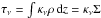 , where κν is the opacity per unit of mass (assumed to be independent of z). The disk is optically thick in the vertical direction up to radii where τν = 1, which is using the continuity equation given by
 ![Mathematical equation: \begin{eqnarray} \label{babice} R&=&\frac{\kappa_\nu\dot M}{2\pi \varv_R}\approx 14\,{R}_\odot\, \zav{\frac{\kappa_\nu}{1\,\text{cm}^2\,\text{g}^{-1}}} \zav{\frac{\dot M}{10^{-10}\,{M}_\odot\,\text{year}^{-1}}} \nonumber\\[2mm] &&\times~ \zav{\frac{\varv_R}{10\,\text{m}\,\text{s}^{-1}}}^{-1}\cdot \end{eqnarray}](/articles/aa/full_html/2015/01/aa24867-14/aa24867-14-eq108.png) (16)The disk is optically thick close to the star for a given frequency, while it becomes optically thin at larger distances, creating some kind of a “pseudo-photosphere” (e.g., Koubský et al. 1997). For example, for a typical disk mass-loss rate 10-10 M⊙ year-1 and electron scattering opacity with κν ≈ 0.4 cm2 g-1, the disk is optically thick only to a few of stellar radii. A similar estimate can be derived for hydrogen bound-free absorption, but this is complicated by the uncertain disk ionization state.
(16)The disk is optically thick close to the star for a given frequency, while it becomes optically thin at larger distances, creating some kind of a “pseudo-photosphere” (e.g., Koubský et al. 1997). For example, for a typical disk mass-loss rate 10-10 M⊙ year-1 and electron scattering opacity with κν ≈ 0.4 cm2 g-1, the disk is optically thick only to a few of stellar radii. A similar estimate can be derived for hydrogen bound-free absorption, but this is complicated by the uncertain disk ionization state.
The free-free absorption likely dominates in the radio domain at large distances from the star. Equation (16)cannot be directly used in this case because of the dependence of the opacity on the density squared. Assuming a hydrostatic density distribution in the vertical direction,  , and χν ≈ κ0ν-3T− 1 / 2ρ2 (Mihalas 1978), the radius at which the vertical optical depth is unity is
  (17)for the free-free absorption. Here we used the continuity equation. In scaled quantities, Eq. (17)reads
 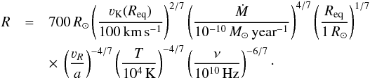 (18)This shows that for realistic disk parameters the extension of Be-star disks in the radio domain is of the order of hundreds of stellar radii, and it does not indicate the outer disk edge. Instead of this, radio observations can be used to determine the disk mass-loss rate.
8. Disks of Be/X-ray binaries
The X-ray emission in the Be/X-ray binaries comes from the accretion of the Be star disk material onto the neutron star (see Reig 2011, for a review). The binary separation D therefore provides a constraint on the outer disk radius, although the process of a disk truncation is complex and there may not be a unique relationship between outer disk radius and the binary separation (Okazaki & Negueruela 2001).
Within the classical Bondi-Hoyle-Littleton approximation, the neutron star accretes from the radius (Waters et al. 1989; Okazaki & Negueruela 2001)  (19)where MX is the neutron star mass and νrel is the relative velocity of the neutron star and the disk. There are two extreme cases for aligned systems, either the neutron accretes material that is corrotating, in which case
  (20a)or the disk is truncated far from the neutron star, in which case the relative velocity may be roughly approximated by
  (20b)If the accretion radius is larger than the disk scale height, racc>H, then the neutron star may accrete all material from the disk, giving the X-ray luminosity
  (21)where RX is the neutron star radius. In the opposite case, racc<H, only a fraction of about racc/H of the disk material is accreted.
In Fig. 5 we compare the accretion radius with disk scale-height for the model displayed in Fig. 1. For both Eqs. (20a)and (20b)the neutron star accretion radius is significantly larger than the disk scale height up to the distance of the order of hundreds of stellar radii from the Be star. We also note that the time needed to cross the distance H in the radial direction H/ νR ≈ (a/ νR)Porb is longer than the local orbital period Porb in the subsonic part of the disk (νR<a). This indicates that the neutron star is able to accrete all material from the disk if the neutron star resides in a subsonic part of the disk. Therefore, with known X-ray luminosity one can infer from Eq. (21)the disk mass-loss rate for aligned systems.
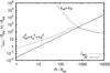 |
Fig. 5 Comparison of the neutron star accretion radius (calculated using Eqs. (20a)and (20b)) with the disk scale height. |
Parameters of Be/X-ray binaries.
In Table 1 we collected a sample of Be/X-ray binaries from literature. In all cases the binary separation is relatively low, therefore the neutron star is able to accrete all material from the disk. From Eq. (21)we derive for stars in Table 1 an estimate of the disk mass-loss rate of the order of 10-13 − 10-9 M⊙ year-1, which quantitatively agrees with theoretical estimates derived from evolutionary calculations of Granada et al. (2013).
The temperature of the disk in Be/X-ray binaries may be affected by the X-ray irradiation. To estimate the influence of this effect, we calculated additional stationary models with radially increasing temperature T = T0(Req/R)p with p< 0. In these models the disk critical point is located closer to the stellar surface than in isothermal disks (cf. Kurfürst et al. 2014). This means that the neutron star is located in the region of the sonic point for many stars in Table 1. For a larger binary separation the neutron star is not able to accrete all material from the disk and the X-ray luminosity should decrease (see Fig. 5). This might be one of the reasons why we do not observe Be/X-ray binaries with very large separation.
9. Discussion
9.1. Influence of the radiative heating and cooling
The derivation of the dispersion relation Eq. (1)assumes adiabatic perturbations. However, the outflowing disks of hot stars can be assumed to be in the radiative equilibrium close to the star (Millar & Marlborough 1998; Carciofi & Bjorkman 2008). In this case it is more natural to assume isothermal instead of adiabatic perturbations. This is frequently done in numerical MRI simulations (e.g., Miller & Stone 2000; Papaloizou & Nelson 2003; Fromang & Nelson 2006), but detailed models include radiation transport (Flaig et al. 2009). These simulations show that MRI and a subsequent turbulence also develops in the case of perturbations in the radiative equilibrium. Consequently, our main conclusions remain the same even for disks in radiative equilibrium.
9.2. Implications for stellar mass-loss
The disk mass-loss rate is determined by the angular-momentum loss needed to keep the star near to the critical rotation. The larger the extension of the disk, the larger the specific angular momentum of the disk material, and the lower the mass-loss rate. Close to the sonic point the disk angular momentum-loss rate flattens (see Fig. 1) and becomes independent of radius. MRI disappears in this region, which means that we can use the sonic point radius to calculate the disk mass-loss rate, as was suggested by Krtička et al. (2011).
9.3. Radial variations of α viscosity parameter
The MRI simulations can be divided into two types. The local ones, confined to a simulation box with a typical dimension of few scale heights (e.g., Hawley & Balbus 1991; Stone et al. 1996) and the global ones (e.g., Hawley & Krolik 2001; Penna et al. 2013). But even the global simulations do not address the problem of the viscosity variations at a distance of the order of hundreds of stellar radii. Consequently, one has to rely on the analytic analysis to estimate the radial behaviour of the viscosity.
The order-of-magnitude viscosity estimate is μ ≈ ρℓ ⟨ v ⟩, where ρ is the density, ℓ is the mean free path, and ⟨ v ⟩ is the mean velocity. The mean free path of the perturbed element can be estimated assuming that the radial scale of turbulent elements is the same as the vertical one, ℓ ≈ H, and the mean velocity can be assumed to be proportional to ⟨ v ⟩ ≈ |ω|ℓ. This gives for the viscosity μ ≈ ρ|ω|H2, which from Eq. (13)depends on radius as μ ~ R-2 close to the star. Equating this to the viscosity parameterization μ ≈ αρHa suggested by Shakura & Sunyaev (1973), we conclude that α does not depend on radius close to the star. This agrees with numerical simulations of Penna et al. (2013). From this discussion it follows that at larger distances one can assume α ≈ |ω|R/ νK.
9.4. Disk extension
Our main results are valid for accretion disks as well. From the discussion here it follows that the decretion or accretion disk extension is of the order of the critical (sonic) point radius. For the isothermal disks Eq. (14) of Krtička et al. (2011) gives 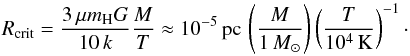 (22)This yields the disk extension of hundreds to thousands of solar radii for disks around objects with mass of the order of the solar mass, while it gives tens to ten thousands of parsec for supermassive black holes found in centres of galaxies.
10. Conclusions
We provided an analytic study of the MRI as a source of anomalous viscosity in Be star disks. Our study needs to be verified by future magnetohydrodynamical simulations, but this does not seem to alter the basic results of our paper:
-
The MRI does not develop in stars with a strong surface magnetic field. In these stars the plasma β parameter is too low and the material is not transported outwards by MRI.
-
The MRI disappears at large distances from the star, where the disk rotational velocity is equal to the sound speed and the radial disk velocity approaches the sound speed. In isothermal disks this occurs at the radius of several hundreds of stellar radii. The time-dependent simulations show that the disks may disseminate to the infinity even in the case of vanishing MRI.
-
The radial dependence of the angular momentum-loss rate flattens at the regions where MRI disappears, consequently the relation between the mass-loss rate and angular-momentum rate (Krtička et al. 2011) is valid in this case.
-
We discussed the observational limits on the outer disk structure for Be and Be/X-ray stars. For Be stars the optical and possibly even radio observations do not trace the outer disk radius. For Be/X-ray binaries the neutron star is able to accrete all material from the disk, which makes the X-ray luminosity a measure of the disk mass-loss rate.
Acknowledgments
This work was supported by the grant GA ČR 13-10589S. The access to computing and storage facilities owned by parties and projects contributing to the National Grid Infrastructure MetaCentrum, provided under the program “Projects of Large Infrastructure for Research, Development, and Innovations” (LM2010005) is appreciated.
References
- Balbus, S. A., & Hawley, J. F. 1991, ApJ, 376, 214 [NASA ADS] [CrossRef] [Google Scholar]
- Barnsley, R. M., & Steele, I. A. 2013, A&A, 556, A81 [NASA ADS] [CrossRef] [EDP Sciences] [Google Scholar]
- Bodaghee, A., Rahoui, F., Tomsick, J. A., & Rodriguez, J. 2012, ApJ, 751, 113 [NASA ADS] [CrossRef] [Google Scholar]
- Caballero, I., Pottschmidt, K., Santangelo, A., et al. 2010, Eighth Integral Workshop. The Restless Gamma-ray Universe (INTEGRAL 2010), 63 [Google Scholar]
- Carciofi, A. C. 2011, IAU Symp., 272, 325 [NASA ADS] [Google Scholar]
- Carciofi, A. C., & Bjorkman, J. E. 2008, ApJ, 684, 1374 [NASA ADS] [CrossRef] [EDP Sciences] [Google Scholar]
- Casares, J., Ribó, M., Ribas, I., et al. 2012, MNRAS, 421, 1103 [NASA ADS] [CrossRef] [Google Scholar]
- Coe, M. J., Bird, A. J., Hill, A. B., et al. 2007, MNRAS, 378, 1427 [NASA ADS] [CrossRef] [Google Scholar]
- Combi, J. A., Ribó, M., Mirabel, I. F., & Sugizaki, M. 2004, A&A, 422, 1031 [NASA ADS] [CrossRef] [EDP Sciences] [Google Scholar]
- Dougherty, S. M., & Taylor, A. R. 1992, Nature, 359, 808 [NASA ADS] [CrossRef] [Google Scholar]
- Ekström, S., Meynet, G., Chiappini, C., Hirschi, R., & Maeder, A. 2008, A&A, 489, 685 [NASA ADS] [CrossRef] [EDP Sciences] [Google Scholar]
- Flaig, M., Kissmann, R., & Kley, W. 2009, MNRAS, 394, 1887 [NASA ADS] [CrossRef] [Google Scholar]
- Fromang, S., & Nelson, R. P. 2006, A&A, 457, 343 [NASA ADS] [CrossRef] [EDP Sciences] [MathSciNet] [Google Scholar]
- Fujii, Y. I., Okuzumi, S., Tanigawa, T., & Inutsuka, S.-I. 2014, ApJ, 785, 101 [NASA ADS] [CrossRef] [Google Scholar]
- Giovannelli, F., Bisnovatyi-Kogan, G. S., & Klepnev, A. S. 2013, A&A, 560, A1 [NASA ADS] [CrossRef] [EDP Sciences] [Google Scholar]
- Granada, A., Ekström, S., Georgy, C., et al. 2013, A&A, 553, A25 [NASA ADS] [CrossRef] [EDP Sciences] [Google Scholar]
- Greiner, J., & Rau, A. 2001, A&A, 375, 145 [NASA ADS] [CrossRef] [EDP Sciences] [Google Scholar]
- Harmanec, P. 1988, Bull. Astron. Inst. Czechosl. 39, 329 [Google Scholar]
- Hawley, J. F., & Balbus, S. A. 1991, ApJ, 376, 223 [NASA ADS] [CrossRef] [Google Scholar]
- Hawley, J. F., & Krolik, J. H. 2001, ApJ, 548, 348 [NASA ADS] [CrossRef] [Google Scholar]
- Hubert, A. M., & Floquet, M. 1998, A&A, 335, 565 [NASA ADS] [Google Scholar]
- Ikhsanov, N. R., Larionov, V. M., & Beskrovnaya, N. G. 2001, A&A, 372, 227 [NASA ADS] [CrossRef] [EDP Sciences] [Google Scholar]
- Janot Pacheco, E., Chevalier, C., & Ilovaisky, S. A. 1982, Be Stars, 98, 151 [NASA ADS] [CrossRef] [Google Scholar]
- Jones, C. E., Tycner, C., & Smith, A. D. 2011, AJ, 141, 150 [NASA ADS] [CrossRef] [Google Scholar]
- Koubský, P., Harmanec, P., Kubát, J., et al. 1997, A&A, 328, 551 [NASA ADS] [Google Scholar]
- Kraus, M., Borges Fernandes, M., & de Araújo, F. X. 2010, A&A, 517, A30 [NASA ADS] [CrossRef] [EDP Sciences] [Google Scholar]
- Krtička, J., Owocki, S. P., & Meynet, G., 2011, A&A, 527, A84 [NASA ADS] [CrossRef] [EDP Sciences] [Google Scholar]
- Kurfürst, P., Feldmeier, A., & Krtička, J. 2014, A&A, 569, A23 [NASA ADS] [CrossRef] [EDP Sciences] [Google Scholar]
- Kühnel, M., Müller, S., Kreykenbohm, I., et al. 2013, A&A, 555, A95 [NASA ADS] [CrossRef] [EDP Sciences] [Google Scholar]
- Lee, U., Osaki, Y., & Saio, H. 1991, MNRAS, 250, 432 [NASA ADS] [CrossRef] [Google Scholar]
- Lignières, F., Petit, P., Böhm, T., & Aurière, M. 2009, A&A, 500, L41 [NASA ADS] [CrossRef] [EDP Sciences] [Google Scholar]
- Martins, F., Schaerer, D., & Hillier, D. J. 2005, A&A, 436, 1049 [NASA ADS] [CrossRef] [EDP Sciences] [Google Scholar]
- Massi, M. 2004, European VLBI Network on New Developments in VLBI Science and Technology, 215 [Google Scholar]
- Meilland, A., Stee, P., Chesneau, O., & Jones, C. 2009, A&A, 505, 687 [NASA ADS] [CrossRef] [EDP Sciences] [Google Scholar]
- Meynet, G., Ekström, S., & Maeder, A. 2006, A&A, 447, 623 [NASA ADS] [CrossRef] [EDP Sciences] [Google Scholar]
- Mihalas, D. 1978, Stellar Atmospheres (San Francisco: Freeman & Co.) [Google Scholar]
- Millar, C. E., & Marlborough, J. M. 1998, ApJ, 494, 715 [NASA ADS] [CrossRef] [Google Scholar]
- Miller, K. A., & Stone, J. M. 2000, ApJ, 534, 398 [NASA ADS] [CrossRef] [Google Scholar]
- Moldón, J., Ribó, M., & Paredes, J. M. 2011, A&A, 533, L7 [NASA ADS] [CrossRef] [EDP Sciences] [Google Scholar]
- Montani, G., Benini, R., Carlevaro, N., & Franco, A. 2013, MNRAS, 436, 327 [NASA ADS] [CrossRef] [Google Scholar]
- Okazaki, A. T. 2001, PASJ, 53, 119 [NASA ADS] [CrossRef] [Google Scholar]
- Okazaki, A. T., & Negueruela, I. 2001, A&A, 377, 161 [NASA ADS] [CrossRef] [EDP Sciences] [Google Scholar]
- Okuzumi, S., & Ormel, C. W. 2013, ApJ, 771, 43 [NASA ADS] [CrossRef] [Google Scholar]
- Papaloizou, J. C. B., & Nelson, R. P. 2003, MNRAS, 339, 983 [NASA ADS] [CrossRef] [Google Scholar]
- Penna, R. F., Sądowski, A., Kulkarni, A. K., & Narayan, R. 2013, MNRAS, 428, 2255 [NASA ADS] [CrossRef] [Google Scholar]
- Petit, P., Lignières, F., Auriére, M., et al. 2011, A&A, 532, L13 [NASA ADS] [CrossRef] [EDP Sciences] [Google Scholar]
- Reig, P. 2011, Ap&SS, 332, 1 [NASA ADS] [CrossRef] [Google Scholar]
- Reig, P., Fabregat, J., Coe, M. J., et al. 1997, A&A, 322, 183 [NASA ADS] [Google Scholar]
- Rivinius, T., Carciofi, A. C., & Martayan, C. 2013, A&A Rev., 21, 69 [Google Scholar]
- Sarty, G. E., Kiss, L. L., Huziak, R., et al. 2009, MNRAS, 392, 1242 [NASA ADS] [CrossRef] [Google Scholar]
- Shakura, N. I., & Sunyaev, R. A. 1973, A&A, 24, 337 [NASA ADS] [Google Scholar]
- Sierpowska-Bartosik, A., & Bednarek, W. 2008, MNRAS, 385, 2279 [NASA ADS] [CrossRef] [Google Scholar]
- Štefl, S., Le Bouquin, J.-B., Carciofi, A. C., et al. 2012, A&A, 540, A76 [NASA ADS] [CrossRef] [EDP Sciences] [Google Scholar]
- Stevens, J. B., Reig, P., Coe, M. J., et al. 1997, MNRAS, 288, 988 [NASA ADS] [CrossRef] [Google Scholar]
- Stone, J. M., Hawley, J. F., Gammie, C. F., & Balbus, S. A. 1996, ApJ, 463, 656 [NASA ADS] [CrossRef] [Google Scholar]
- Sushch, I., de Naurois, M., Schwanke, U., Spengler, G., & Bordas, P. 2012, Fermi Symp. proc. – eConf C121028 [Google Scholar]
- Thompson, T. W. J., Tomsick, J. A., Rothschild, R. E., in’t Zand, J. J. M., & Walter, R. 2006, ApJ, 649, 373 [NASA ADS] [CrossRef] [Google Scholar]
- Touhami, Y., Gies, D. R., Schaefer, G. H., et al. 2013, ApJ, 768, 128 [NASA ADS] [CrossRef] [Google Scholar]
- ud-Doula, A., Owocki, S. P., & Townsend, R. H. D. 2009, MNRAS, 392, 1022 [NASA ADS] [CrossRef] [Google Scholar]
- Waters, L. B. F. M., de Martino, D., Habets, G. M. H. J., & Taylor, A. R. 1989, A&A, 223, 207 [NASA ADS] [Google Scholar]
- Zamanov, R. K., & Martí, J. 2000, IAU Colloq. 175: The Be Phenomenon in Early-Type Stars, 214, 731 [NASA ADS] [Google Scholar]
- Zamanov, R., Marti, J., & Marziani, P. 2001, The Second National Conference on Astrophysics of Compact Objects, 50 [Google Scholar]
All Tables
All Figures
|
Fig. 1 Dependence of the radial and azimuthal velocities (in units of sound speed a), the midplane disk density ρ0 (relative to its value at R = Req), the angular momentum-loss rate in units of equator release angular momentum-loss rate |
| In the text | |
|
Fig. 2 Zero-crossing root of the dispersion relation Eq. (1)as a function of radial and vertical wavenumbers at R = 1.01 Req for the model given in Fig. 1. The plane ω = 0 divides perturbations that are stable − ω2< 0 from that leading to an instability − ω2> 0. The red region denotes perturbations with a too large characteristic scale that can not be accommodated in the disk |
| In the text | |
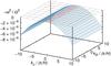 |
Fig. 3 Same as Fig. 2, but for R = 440 Req. |
| In the text | |
|
Fig. 4 Final stationary state of time-dependent disk models with constant and variable viscosity parameter α. We plot the same variables as in the stationary model in Fig. 1. In the constant-viscosity model (dashed line) the viscosity parameter α = α(Req), while in the decreasing-viscosity model (solid line) the parameter α = α(Req)[ (391 Req − R) / (390 Req) ] below R = 390 Req and α = α(Req) / 390 elsewhere. The inner boundary viscosity parameter α(Req) = 0.1. We consider the isothermal disk of the main-sequence B2–B3 type star (see Sect. 3). Arrows denote the locations of the critical points. |
| In the text | |
|
Fig. 5 Comparison of the neutron star accretion radius (calculated using Eqs. (20a)and (20b)) with the disk scale height. |
| In the text | |
Current usage metrics show cumulative count of Article Views (full-text article views including HTML views, PDF and ePub downloads, according to the available data) and Abstracts Views on Vision4Press platform.
Data correspond to usage on the plateform after 2015. The current usage metrics is available 48-96 hours after online publication and is updated daily on week days.
Initial download of the metrics may take a while.