| Issue |
A&A
Volume 573, January 2015
|
|
|---|---|---|
| Article Number | A102 | |
| Number of page(s) | 7 | |
| Section | Planets and planetary systems | |
| DOI | https://doi.org/10.1051/0004-6361/201423687 | |
| Published online | 06 January 2015 | |
An updated estimate of the number of Jupiter-family comets using a simple fading law
1 Earth-Life Science Institute, Tokyo Institute of Technology, Meguro, 152-8551 Tokyo, Japan
e-mail: brasser_astro@yahoo.com
2 Institute for Astronomy and Astrophysics, Academia Sinica; 11F AS/NTU building, 1 Roosevelt Rd., Sec. 4, 10617 Taipei, Taiwan
Received: 21 February 2014
Accepted: 27 October 2014
It has long been hypothesised that the Jupiter-family comets (JFCs) come from the scattered disc, an unstable planetesimal population beyond Neptune. This viewpoint has been widely accepted, but a few issues remain, the most prominent of which are the total number of visible JFCs with a perihelion distance q < 2.5 AU and the corresponding number of objects in the scattered disc. In this work we give a robust estimate of the number of visible JFCs with q < 2.5 AU and diameter D> 2.3 km based on recent observational data. This is combined with numerical simulations that use a simple fading law applied to JFCs that come close to the Sun. For this we numerically evolve thousands of comets from the scattered disc through the realm of the giant planets and keep track of their number of perihelion passages with perihelion distance q < 2.5 AU, below which the activity is supposed to increase considerably. We can simultaneously fit the JFC inclination and semi-major axis distribution accurately with a delayed power law fading function of the form Φm ∝ (M2 + m2)− k/ 2, where Φm is the visibility, m is the number of perihelion passages with q < 2.5 AU, M is an integer constant, and k is the fading index. We best match both the inclination and semi-major axis distributions when k ~ 1.4, M = 40, and the maximum perihelion distance below which the observational data is complete is qm ~ 2.3 AU. From observational data we calculate that a JFC with diameter D = 2.3 km has a typical total absolute magnitude HT = 10.8, and the steady-state number of active JFCs with diameter D > 2.3 km and q < 2.5 AU is of the order of 300 (but with large uncertainties), approximately a factor two higher than earlier estimates. The increased JFC population results in a scattered disc population of 6 billion objects and decreases the observed Oort cloud to scattered disc population ratio to 13, virtually the same as the value of 12 obtained with numerical simulations.
Key words: comets: general
© ESO, 2015
1. Introduction
The solar system is host to a large population of comets, which tend to be concentrated in three reservoirs: the Oort cloud (Oort 1950), the Kuiper belt and scattered disc (Duncan & Levison 1997). The third is the source of the so-called Jupiter-family comets (JFCs), a population of comets whose orbits stay close to the ecliptic (Duncan & Levison 1997; Volk & Malhotra 2008; Brasser & Morbidelli 2013). In this study we adhere to the definition of Levison (1996) which states that a JFC has TJ ∈ (2,3) and a < 7.35 AU (period P < 20 yr). Here a is the semi-major axis and TJ is the Tisserand parameter with respect to Jupiter. In addition, we impose a perihelion distance q < 5 AU. By contrast, the Oort cloud is the source of the Halley-type comets (HTCs, Wang & Brasser 2014), which are defined as having TJ < 2 and P < 200 yr (Levison 1996). The long-period comets (LPCs) have P> 200 yr.
The origin and dynamical evolution of the JFCs have been intensively investigated. Levison & Duncan (1997) ran many numerical simulations in which they evolved test particles from the Kuiper belt through the realm of the giant planets until they became visible JFCs (which are defined as JFCs with perihelion distance q < 2.5 AU). They found that approximately 30% of Kuiper belt objects became JFCs. The JFC inclination distribution could only be reproduced if the comets faded or disintegrated after a total active lifetime of 12 kyr. This implied that the JFCs spent about 3 kyr, or about 400 returns, while active with q < 2.5 AU. Levison & Duncan (1997) conclude that in steady-state there should be approximately 100 JFCs with diameter D> 2 km and q < 2.5 AU.
Their work was followed by Duncan & Levison (1997) who concluded that the scattered disc and not the Kuiper belt had to produce the JFCs, a conclusion that was confirmed in subsequent works by Emel’yanenko et al. (2004), Volk & Malhotra (2008), and Brasser & Morbidelli (2013). Duncan & Levison (1997) also reported that the scattered disc had to contain 6 × 10⁸ objects with diameter D> 2 km, confirmed by Volk & Malhotra (2008).
Fernández et al. (2002) studied the evolution of JFCs in parallel to the above works, and reproduced the median dynamical lifetime and physical lifetimes reported in Levison & Duncan (1997). Their work was superseded by that of Di Sisto et al. (2009), who employed an elaborate splitting and fading mechanism to constrain the JFC population and reproduce the orbital element distributions. They conclude that the active lifetime is comparable to that found by Duncan & Levison (1997) and Fernández et al. (2002) and that in steady state there are approximately 100 JFCs with diameter D> 2 km and q < 2.5 AU.
Despite the above successes in reproducing the orbital distribution and number of the JFC population several issues remain. Wang & Brasser (2014) successfully reproduced the orbital distribution of the HTCs by employing a simple fading law. Here we apply the same fading law and techniques to numerical simulations of JFC production, and determine whether this reproduces their orbital distribution and the increase in total absolute magnitude determined from observations. We use the results of the fading law to update the number of JFCs with a diameter larger than 2.3 km estimated in Brasser & Morbidelli (2013). This paper is organised as follows.
In the next section we briefly discuss the observational dataset that we employed. In Sect. 3 we use the observed absolute magnitudes and sizes of JFC nuclei to determine their active fraction and the increase in total absolute magnitude from a fully active comet. Section 4 contains a summary of the numerical simulations that we performed. In Sect. 5 we discuss the results, Sect. 6 discusses an important implication of our work. A discussion follows in Sect. 7 and we draw our conclusions in the last section.
2. Observational dataset
In this study we determine whether the orbital distribution of the JFCs can be obtained by using a similar simple fading law that was applied to the HTCs in Wang & Brasser (2014), and to update the number of active JFCs with q < 2.5 AU. Since the JFCs originate in scattered disc (Duncan & Levison 1997; Emel’yanenko et al. 2004; Volk & Malhotra 2008; Di Sisto et al. 2009; Brasser & Morbidelli 2013), we also update the inferred number of scattered disc objects (SDOs) by using the total number of active JFCs as a proxy. To compare our simulation with the observational data we need to have an observational catalogue of comets that is as complete as possible. Just as in Wang & Brasser (2014) we chose to use the JPL Small-Body Search Engine1.
In total the catalogue contains 406 JFCs.
In addition to their orbital parameters we want to obtain an estimate of the number of JFCs as a function of their size. To do so requires knowledge of both the total absolute magnitude and the nuclear absolute magnitudes of all the comets or their diameters. The most complete set of JFC nucleus sizes was reported in Snodgrass et al. (2011) and the most comprehensive list of total absolute magnitudes is from Kresak & Kresakova (1994). Using these combined works the total number of JFCs for which both the total absolute magnitude and diameter are known is 68. We make use of these in Sect. 5.
3. Absolute magnitude of JFCs versus LPCs
Based on the data from Fernández et al. (1999) and Fernández & Morbidelli (2006), Brasser & Morbidelli (2013) estimated that a JFC with D = 2.3 km has an absolute magnitude of approximately HT = 9.3. Here we aim to make a more accurate estimate based on available observational data.
Fernández et al. (1999) derive several relations between the total brightness, BT, and diameter of JFCs, D, and the fraction of the surface that shows active outgassing, f. If the magnitude limit of the coma is set by its fading into the sky background – applicable to more distant and smaller comet nuclei and low-active comets – they obtain BT ∝ f2D3. However, for comets whose coma is larger than the aperture of the telescope BT ∝ fD3/2, while BT ∝ fD5/2 for comets far from the Sun where the activity decreases substantially. A priori it is difficult to know which relation to choose, but generally it appears to be BT ∝ fDδ with 3/2 <δ < 5/2. Figure 1 depicts the total absolute magnitude of those JFCs for which their diameters are known. There are a few outliers with D> 10 km that were excluded. The absolute magnitudes were taken from Kresak & Kresakova (1994) and the diameters are from Snodgrass et al. (2011). The lines show the diameter-magnitude relation for various values of f. From bottom to top these are 1, 0.1, 0.01 and 0.001. From the figure and the available data typically f ~ 0.01 when BT ∝ fDδ, and f ~ 0.2 when BT ∝ f2D3. Are these D − HT relations and values of f for JFCs consistent with observational data?
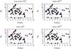 |
Fig. 1 Scatter plot of the diameter versus total absolute magnitude of JFCs. The absolute magnitudes come from Kresak & Kresakova (1994) and the diameters are taken from Snodgrass et al. (2011). The lines show the diameter-magnitude relation for various values of f. From bottom to top these are f = 1, 0.1, 0.01, and 0.001. |
Fernández (2005) states that for a JFC the typical value of f is around 0.02. To verify this we computed log f for all the comets in Fig. 1. This was done as follows. For the remainder of the paper we assume that BT ∝ fD2 and thus  (1)with
  being a constant. In theory a completely inactive comet has f = 0, but then Eq. (1) is no longer valid. In practice a minimum value of f is attained when HT is equal to the absolute magnitude of the bare nucleus, which occurs typically when fmin ~ 10-4. We need to calibrate the constant , but since the active fraction of JFCs is unknown we need to rely on a population of comets where the active fraction is known. These are the LPCs.
From Sosa & Fernández (2011) we have for the LPCs HT = 9.3−7.7 log D and when D = 2.3 km HT = 6.5. Equating this to Eq. (1) and setting f = 1 we find that  . Now we can compute f as a function of HT and D for the JFCs whose total absolute magnitude and diameter are known. We find log f follows a Gaussian distribution with ⟨ log f ⟩ = −1.73 and standard deviation σ = 0.83. This reinforces the notion that the JFCs are much less active than LPCs of the same size and also invalidates the relation BT ∝ f2D3 for these comets. The change in f needs to be converted into a change in total absolute magnitude, ΔHT.
With each perihelion passage with q < 2.5 AU the comet loses mass. One may follow di Sisto et al. (2009) to compute how much mass is lost per perihelion passage, but the end result is the same: the comet fades by reducing the diameter through sublimation and the active fraction through the formation of insulating layers (Rickman et al. 1990, 1991). The reduction in diameter and active surface fraction yields a change in absolute magnitude ΔHT = −5log (Di/Df) − 2.5log (fi/ff), where subscript i stands for initial values and subscript f for final values. When one considers a typical mass loss rate of 40 g cm-2 per perihelion passage (Fernández 2005), which occurs when q ~ 2 AU, then after a few hundred passages for small comets log (Df/Di) ~ − 0.1 and, assuming the active fraction stays constant, ΔHT ~ 0.5.
However, the active fraction does not stay constant but decreases as well, most likely in accordance with the crust building scenario. From Fig. 1 many observed JFCs have f ~ 0.01–0.1. Assuming that fi ~ 1 like the LPCs and that after substantial orbital evolution ff is in this range, we have ΔHT = 2.5–5 mag. This range of increased absolute magnitude is consistent with earlier estimates by Whipple (1978) but lower than those of Fernández et al. (1999) and Fernández & Morbidelli (2006). Generally, the increase in total absolute magnitude is closer to the upper end than the lower one. In other words, the greatest increase in the absolute magnitude, i.e. the fading, is caused by the active fraction of the comet decreasing. A caveat could exist in assuming fi ~ 1, but since we observe some JFCs with a very high active fraction, these are most likely young comets (Rickman et al. 1991) and thus this assumption appears justified.
In conclusion, a typical JFC is about ΔHT = −2.5 × − 1.73 = 4.3 mag fainter than an LPC of the same size. This is much fainter than what was used in Brasser & Morbidelli (2013). We now need to find a fading law that fits the semi-major axis and inclination distributions of the JFCs, and simultaneously matches the observed amount of fading. The methodology is discussed in the next sections.
4. Numerical simulation and initial conditions
The numerical simulations and initial conditions for this study are described in detail in Brasser & Morbidelli (2013). In that work they modelled the formation of the Oort cloud and scattered disc during an episode of giant planet instability. They used the giant planet evolution of Levison et al. (2008) for the phase of giant planet migration and then continued to evolve the system for an additional 4 Gyr, stopping and resuming a few times to clone remaining particles for statistical reasons. However, for this study we had to rerun the last 500 Myr of the scattered disc with the same code that was used in Wang & Brasser (2014) to obtain the number of perihelion passages with time of any JFCs we might have produced. For these simulations we used SCATR (Kaib et al. 2011). We set the boundary between the regions with short and long time step at 300 AU from the Sun (Kaib et al. 2011). Closer than this distance the computations are performed in the heliocentric frame with a time step of 0.1 yr. Farther than 300 AU, the calculations are performed in the barycentric frame and we increased the time step to 50 yr. Comets were removed once they were farther than 1000 AU from the Sun, or if they collided with the Sun or a planet. The terrestrial planets were not included because they only have a minimal effect on the dynamics of the JFCs (Levison et al. 2006a) and they would increase computation time by at least an order of magnitude.
To determine how the comets fade we modified SCATR to keep track of the number of perihelion passages of each comet. By fading we mean that the comets’ visibility (or brightness) decreases. This could be caused by actual fading, splitting, or development of an insulating crust. Levison et al. (2001) suggest that comets fade the most quickly when their perihelion distance q < 2.5 AU, which is the distance at which water ice begins to sublimate, so we only counted the number of perihelion passages when the perihelion was closer than 2.5 AU.
We applied a post-processing fading law, Φm, which is a function of the number of perihelion passages, m. Here Φm is the remaining visibility function introduced by Wiegert & Tremaine (1999). A comet that has its mth perihelion passage with q < 2.5 AU will have its remaining visibility be Φm up to m = np, where np is the maximum number of perihelion passages before dynamical elimination by Jupiter; in addition Φ1 = 1 for the first out-going perihelion passage of a comet, Without fading, every comet in our simulation has the same weighting (Φm = 1,m = 1,2,3...,np) in constructing the cumulative distribution of semi-major axis or inclination of active comets. When we imposed the fading effect to comets, the remaining visibility Φm is considered as a weighting factor. The higher the number of perihelion passages, the less each comet contributes to the cumulative inclination or semi-major axis distribution of the active comets because of fading.
In order to find out how well our simulations match with the observed JFCs we follow Wang & Brasser (2014). We computed the cumulative inclination and semi-major axis distributions of the observed and simulated comets. In each case we imposed a maximum perihelion distance, qm, below which we deem the observational sample to be complete, and employed several functional forms of Φm. Once these distributions were generated we performed a Kolmogorov-Smirnov (K-S) test (Press et al. 1992), which searches for the maximum absolute deviation dmax between the observed and simulated cumulative distributions. The K-S test assumes that the entries in the distributions are statistically independent. The probability of a match, Pd, as a function of dmax, can be calculated to determine whether these two populations were drawn from the same parent distribution. However, in our simulations, a single comet would be included many times in the final distribution as long as the comet met our criteria for being a JFC during each of its perihelion passages. Including its dynamical evolution in this manner would cause many of the entries in the final distribution to become statistically dependent and the K-S test would be inapplicable.
We solved this problem by applying a Monte Carlo method to perform the K-S test as described in Levison et al. (2006b). Once we have the inclination and semi-major axis distributions from the simulation, we then randomly selected 10 000 fictitious samples from the simulation. Each sample has the same number of data points as JFCs from JPL catalogue. The Monte Carlo K-S probability is then the fraction of cases that have their d values between the fictitious samples and real JFC samples larger than the dmax found from the real JFC samples and cumulative distributions from simulation.
However, before making the fictitious datasets, we need to find the empirical probability density functions of inclination and semi-major axis from which we then sample the fictitious JFCs. Here we generated these from a normalised histogram. One crucial point in making the histogram is that we weighed each entry by its remaining visibility. The fictitious comets were then sampled from the distributions with the von Neumann rejection technique (von Neumann 1950). This sampling method relies on generating two uniform random numbers on a grid. An entry is accepted when both numbers fall under the probability density curve.
5. Results
During the course of investigation we have tried many different forms of Φm, but it was necessary to meet a few requirements. First, the resulting inclination and semi-major axis distributions of the simulated JFCs need to be consistent with the observed sample up to a maximum perihelion distance q < 2.5 AU. Second, the decay needs a fairly short half-life. The half-life is the number of revolutions by which time the visibility, or active surface, has dropped by 50%. This is equivalent to an increase in the total absolute magnitude of 0.75. There are several works that indicate how the comets may decrease their visibility.
Rickman et al. (1991) studied the fading of comets through orbital changes caused by non-gravitational forces. They reported that young, active comets build up an insulating layer in 10 to 20 revolutions and that the brightness of these comets decreases by a factor of four within the same number of revolutions. This suggests the fading happens rather quickly. Simultaneously, Prialnik & Mekler (1991) clearly show that comets fade quickly during the first few returns and much more slowly thereafter. This confirms that comets should fade substantially during the first 10 to 20 revolutions. However, both studies only considered pristine comets where evaporation occurred at a steady rate, while it is known that these same comets build up an insulating layer farther from the Sun (Fernández 2005) which could slow the fading down. Thus we need a fading function with a reasonably slow initial decay that speeds up later.
From our simulations we determined ⟨ log np ⟩ = 2.62 ± 0.85. Thus, a JFC typically passes through perihelion with q < 2.5 AU  times before Jupiter eliminates it. Assuming no gradual fading, the total active lifetime
  kyr, where we used the median orbital period of 7.3 yr, consistent with earlier estimates. Hence after a few hundred revolutions the fading function should match the current typical observed active fraction. We observe both new and old JFCs and thus we assume that a new JFC with m = 1 has the same absolute magnitude as an LPC of the same size, i.e. fi = 1. That said, we want to post one word of caution.
In our simulations a comet is eliminated from the visible region by collision with a planet or the Sun, or by ejection by Jupiter. In addition to these, fading may be in itself an end state since, as comets lose matter, they follow a progressive process of disintegration, leaving meteoritic matter disseminated through interplanetary space as remains of the parent comet, before ejection by Jupiter. Thus, there are additional loss mechanisms apart from planetary ejection. In this regard, the average expected decrease in brightness of 4.3 mag before dynamical ejection can only apply to those members of the population that are large enough to withstand this fading unscathed until Jupiter can eject them. With this caveat in mind we subsequently explore several functional forms of the fading law and their implications.
5.1. Simple power law
The results of applying a fading function of the form Φm = m− k to the simulated JFCs are shown in Fig. 2. Here, and in subsequent figures, we plot contours of the product of the K-S probabilities for the inclination distribution and semi-major axis distribution as a function of qm vertically and another variable (in this case k) horizontally. In this manner we clearly show where the maxima are for both the inclination and semi-major axis distributions simultaneously. We find that the combination of qm and k that best fits both the semi-major axis and inclination distribution is qm = 2.25 AU, k = 0.65 with a combined K-S probability of 39% (comprised of 60% for the semi-major axis and 66% for the inclination). This result suggests the observational sample is complete up to q = 2.25 AU. We also note that the probability maxima lie along a band that shifts towards larger k with decreasing q. This is expected because comets that venture closer tend to evolve faster.
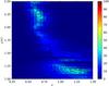 |
Fig. 2 Contour plots of the combined inclination and semi-major axis K-S probability as a function of the fading parameter and maximum perihelion distance for the simple power law. The parameters that best fit both distributions are k = 0.65 and qm = 2.25 AU. |
There is a second maximum at qm = 1.15 AU and k = 1.25. Here the fit for the semi-major axis distribution is very good – although there are few comets to fit the data to – but the inclination match is poor.
What about the total absolute magnitude? Fading causes the total absolute magnitude to increase via ΔHT = −2.5log Φm = 2.5klog m. Using  AU and k = 0.65, after ⟨ np ⟩ revolutions the comets have faded by ΔHT = 4.3 ± 1.4 magnitudes, the same value as was computed in Sect. 3 from observational data. On the other hand, for the other maximum with
  AU and k = 1.25 we need to compute the number of revolutions with q < 1.15 AU. From the perihelion distribution of visible comets the number of JFCs with q < 1.15 AU is just 12% of the number with q < 2.5 AU, from which we compute that ΔHT = 5.4 mag, at least one magnitude higher than for the other maximum. Thus, we report that only the first is consistent with the observational data because the second gives too strong a fading. Unfortunately, even though the power law gives an excellent fit to the data for certain values of qm and k, the half-life is just N1/2 = 21 /k ~ 3 revolutions, which is much shorter than that advocated by Rickman et al. (1991). For this reason we must discard it in favour of a better form.
5.2. Constant fading probability
Chen & Jewitt (1994) suggest that 1% of JFCs are destroyed through splitting per perihelion passage. This fading law is identical to one suggested by Wiegert & Tremaine (1999), which is constant fading probability Φm = (1 − λ)m − 1, where λ is the probability of fading (in this case splitting). We proceeded to search for the value of λ that fit the orbital distribution of the observed JFCs. This is depicted in Fig. 3. Once again there are two maxima, one being much higher than the other. The best fit, with combined K-S probability 42% (91% and 47% for inclination and semi-major axis) has AU and λ = 0.001. Unfortunately, this low splitting or fading probability is inconsistent with the dynamical simulations because the low probability suggests that the comets’ active lifetime is longer than their dynamical lifetime, which is untrue. In other words it does not produce the required amount of fading. After ⟨ np ⟩ revolutions we have  . Imposing λ = 0.01 to be consistent with Chen & Jewitt (1994) does not yield a strong enough fading at the maximum probability near 1.1 AU because the comets only spend 10% of the time with q < 1.1 AU compared to the time they spend with q < 2.5 AU, so that ΔHT ~ 1.4.
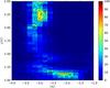 |
Fig. 3 Contour plots of the combined inclination and semi-major axis K-S probability as a function of the fading parameter and maximum perihelion distance for the constant fading probability case. The x-axis is log λ. The parameters that best fit both distributions are λ ~ 0.001 and qm = 2.25 AU. |
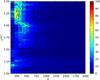 |
Fig. 4 Contour plots of the combined inclination and semi-major axis K-S probability as a function of the fading parameter and maximum perihelion distance for the stretched exponential. The stretching parameter is k = 0.2. The parameters that best fit both distributions are M = 200 and qm = 2.25 AU. |
5.3. Stretched exponential
We next tried a two-parameter fading law of the form Φm = exp [ − (m/M)k], which is called the stretched exponential law, and M is an integer constant. When the stretching parameter k < 1 the population suffers infant mortality, while with k> 1 the population suffers from aged mortality. We found that this fading law is able to reproduce the orbital structure at qm = 2.25 AU and several combinations of M and k. One example is shown in Fig. 4 with k = 0.2, showing the combined K-S probability of semi-major axis and inclination as a function of qm and M. In the example, the highest combined K-S probability is 63% (66% for the semi-major axis and 95% for the inclination). All of the combinations of  , M, and k result in a reasonable fading half-life N1/2 = M(ln2)1 /k ~ 32 revolutions, but unfortunately the fading at high m falls off too slowly to be reconciled with the low active surface fraction of typical JFCs: after ⟨ np ⟩ revolutions we typically have ΔHT = 1.09(np/M)k ~ 1.2 ± 0.4.
5.4. Delayed power law
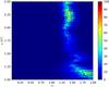 |
Fig. 5 Contour plots of the combined inclination and semi-major axis K-S probability as a function of the fading parameter and maximum perihelion distance for the delayed power law. Here log M = 1.6. The parameters that best fit both distributions are k = 1.4 and qm = 2.30 AU. |
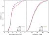 |
Fig. 6 Inclination and semi-major axis distributions from observation and simulation for JFCs that gave the best match from the delayed power law of Fig. 5. |
The last form we tried was the delayed power law  (2)where M is an integer constant. The numerator is chosen to make Φ1 = 1 and at large m the fading proceeds more or less as a power law with m− k. Once again there are several combinations of M and k that yield good fits. The best fit has M = 40, the probability maximum occurs at qm = 2.3 AU and k = 1.4 and is shown in Fig. 5. The combined maximum probability is 53% (35% for inclination and 68% for semi-major axis) and the fits to the cumulative semi-major axis and inclination distributions are depicted in Fig. 6. The left panel shows the semi-major axis distribution, the right panel depicts the inclination distribution. The median simulated inclination is 12.0° (observed 12.4°) and the median simulated semi-major axis is 3.74 AU (observed 3.75 AU). The half-life
  revolutions, longer than the 10 to 20 advocated by Rickman et al. (1991) and Prialnik & Mekler (1991), but this is likely no problem because of the formation of an insulating dust layer. After ⟨ np ⟩ revolutions the comet has faded by ΔH ≈ 2.5klog (M/np) ~ 3.6 ± 2.8 mag, comparable to the estimation from observations but on the low side. Thus, we conclude that this fading law is the most promising because it yields both a high K-S probability, a reasonable match to the total active fraction and has a reasonably long half-life. In conclusion, we suggest that the JFCs fade according to this delayed power law. In the section below we look at the implications of these results.
6. Implication: expected JFC and SDO populations
We can use the results from the numerical simulations above to constrain the expected number of JFCs larger than a given size, building on Levison & Duncan (1997) and Brasser & Morbidelli (2013).
In the last few decades many faint JFCs were discovered with dedicated surveys such as LINEAR, Catalina, Spacewatch, Pan-STARRS, that are not included in Kresak & Kresakova (1994), increasing the average total absolute magnitude of the JFC sample. We can now recompute the total number of JFCs with q < 2.5 AU and D> 2.3 km. From a detailed study of the nuclei and activities of a large sample of JFCs, Fernández et al. (2013) conclude that the JFC population is rather incomplete even for objects with D> 6 km and q < 2 AU. Thus, we need to base our analysis on a sample that is most likely to be complete.
We know from the study by Sosa & Fernández (2011) that an LPC with diameter D = 2.3 km has HT = 6.5, and from observational data presented in Sect. 3 a JFC is approximately 4.3 mag fainter than an LPC of the same size. Therefore, a JFC with D = 2.3 km should typically have a total absolute magnitude of HT = 6.5 + 4.3 = 10.8 rather than HT ~ 9 as was assumed in Levison & Duncan (1997) and Brasser & Morbidelli (2013).
Fernández & Morbidelli (2006) state that there are eight JFCs with HT < 9 and q < 1.3 AU. A subsequent search through recently-discovered JFCs has increased this number to 10. From our simulations and the observational data we find that the fraction of JFCs with q < 1.3 AU is 18% of those with q < 2.5 AU, and thus the number of JFCs with q < 2.5 AU and HT < 9 is 56. We now need to compute the number of JFCs with q < 2.5 AU and HT < 10.8 from the absolute magnitude distribution.
The cumulative total absolute magnitude distribution of the comets obeys N( <HT) ∝ 10− αTHT. Since we have imposed that the total brightness of the comets scales as BT ∝ fD2, it is easy to show that the slope of the total absolute magnitude distribution, αT, is equal to the slope of the nuclear absolute magnitude distribution, α. The latter is related to the cumulative size-frequency distribution, N( >D) ∝ D− γ, where γ = 5α. Even though there is a lot of scatter in the D − HT diagram caused by variation in f from one comet to the next (Fernández et al. 1999), there is a clear correlation between D and HT in Fig. 1 which must be caused by the underlying size distribution. For JFCs with diameters between approximately 2 km and 10 km the slope γ ~ 2 (Meech et al. 2004; Snodgrass et al. 2011), corresponding to α = 0.4. The number of JFCs with q < 2.5 AU and HT < 10.8 is then  , about three times higher than the number reported in Levison & Duncan (1997) and Di Sisto et al. (2009). This is likely to be a lower limit because of the aforementioned incompleteness. However, the fading alters the mean active lifetime, τvFJC, as well. From the output of our simulations and using the delayed power law we computed a weighted mean period of JFCs with q < 2.5 AU of 7.94 yr and a corresponding active lifetime
  yr, lower than previous estimates (Di Sisto et al. 2009; Duncan & Levison 1997; Fernández et al. 2002). Following Brasser & Morbidelli (2013) the corresponding number of objects in the scattered disc with this updated active lifetime, taking into account the uncertainties in all relevant quantities, is then
 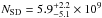 . That same work computed an Oort cloud population of NOC = (7.6 ± 3.3) × 1010 for objects with D> 2.3 km. From our new analysis the Oort cloud to scattered disc population ratio turns out to be 13
 , which is consistent with the ratio of 12 ± 1 from simulations (Brasser & Morbidelli 2013). Thus, it is likely that the Oort cloud and scattered disc formed at the same time from the same source, and thus is consistent with a formation during the giant planet instability.
7. Summary and conclusions
We have performed numerical simulations of the evolution of SDOs until they became visible JFCs. We kept track of their number of perihelion passages with q < 2.5 AU and subsequently imposed a form of fading that depended on the number of revolutions. We computed the cumulative semi-major axis and inclination distributions and found that these match the observed ones from the JPL catalogue when the fading obeys a delayed power law with fading index k = 1.4, a delay of M = 40 and the maximum perihelion is 2.3 AU.
From our simulations we find good agreement of the active lifetime of a JFC with earlier works. Our fading law suggests that a typical JFC has faded by about 3.6 mag before it is eliminated from the solar system by Jupiter or collides with a planet or the Sun, ignoring other loss mechanisms such as disintegration and complete evaporation. This increase in ΔHT is consistent with observational data detailing the active fraction of comets but on the low end. The underlying assumption is that the total brightness of the nucleus and coma follows the relation BT ∝ fD2. The above findings imply that the total absolute magnitude of a JFC with diameter D = 2.3 km is 10.8 rather than 9.3 as reported in Levison & Duncan (1997) and Brasser & Morbidelli (2013). This decreased brightness implies there is an increase in the number of JFCs with D = 2.3 km to approximately 300 rather than the typical 100 estimated elsewhere. With this updated estimate the number of SDOs reaches nearly 6 billion and the Oort cloud to scattered disc population ratio is estimated to be 13, virtually the same as the simulated value of 12 (Brasser & Morbidelli 2013).
Acknowledgments
We thank Paul Weissman for stimulating discussions that greatly improved this manuscript, Alessandro Morbidelli for pointing out an error and Julio Fernández for a review.
References
- Brasser, R., & Morbidelli, A. 2013, Icarus, 225, 40 [NASA ADS] [CrossRef] [Google Scholar]
- Chen, J., & Jewitt, D. 1994, Icarus, 108, 265 [NASA ADS] [CrossRef] [Google Scholar]
- Duncan, M. J., & Levison, H. F. 1997, Science, 276, 1670 [NASA ADS] [CrossRef] [PubMed] [Google Scholar]
- Emel’yanenko, V. V., Asher, D. J., & Bailey, M. E. 2004, MNRAS, 350, 161 [NASA ADS] [CrossRef] [Google Scholar]
- Fernández, J. A. 2005, Comets – Nature, Dynamics, Origin, and their Cosmogonical Relevance (Springer Verlag), Astrophys. Space Sci. Lib., 328 [Google Scholar]
- Fernández, J. A., & Morbidelli, A. 2006, Icarus, 185, 211 [NASA ADS] [CrossRef] [Google Scholar]
- Fernández, J. A., Tancredi, G., Rickman, H., & Licandro, J. 1999, A&A, 352, 327 [NASA ADS] [Google Scholar]
- Fernández, J. A., Gallardo, T., & Brunini, A. 2002, Icarus, 159, 358 [NASA ADS] [CrossRef] [Google Scholar]
- Fernández, Y. R., Kelley, M. S., Lamy, P. L., et al. 2013, Icarus, 226, 1138 [NASA ADS] [CrossRef] [Google Scholar]
- Hughes, D. W. 2001, MNRAS, 326, 515 [Google Scholar]
- Kaib, N. A., Quinn, T., & Brasser, R. 2011, AJ, 141, 3 [NASA ADS] [CrossRef] [Google Scholar]
- Kresak, L., & Kresakova, M. 1994, Planet. Space Sci., 42, 199 [NASA ADS] [CrossRef] [Google Scholar]
- Levison, H. F. 1996, in Completing the Inventory of the solar system, eds. T. Rettig, & J. M. Hahn, ASP Conf. Ser., 107, 173 [Google Scholar]
- Levison, H. F., & Duncan, M. J. 1994, Icarus, 108, 18 [NASA ADS] [CrossRef] [Google Scholar]
- Levison, H. F., & Duncan, M. J. 1997, Icarus, 127, 13 [Google Scholar]
- Levison, H. F., Dones, L., & Duncan, M. J. 2001, AJ, 121, 2253 [NASA ADS] [CrossRef] [Google Scholar]
- Levison, H. F., Terrell, D., Wiegert, P. A., Dones, L., & Duncan, M. J. 2006a, Icarus, 182, 161 [NASA ADS] [CrossRef] [Google Scholar]
- Levison, H. F., Duncan, M. J., Dones, L., & Gladman, B. J. 2006b, Icarus, 184, 619 [NASA ADS] [CrossRef] [Google Scholar]
- Levison, H. F., Morbidelli, A., Van Laerhoven, C., Gomes, R., & Tsiganis, K. 2008, Icarus, 196, 258 [NASA ADS] [CrossRef] [Google Scholar]
- Marsden, B. G., & Williams, G. V. 2008, Catalogue of Cometary Orbits, 17th edn., the International Astronomical Union, Minor Planet Center and Smithsonian Astrophysical Observatory, Cambridge, MA [Google Scholar]
- Meech, K. J., Hainaut, O. R., & Marsden, B. G. 2004, Icarus, 170, 463 [NASA ADS] [CrossRef] [Google Scholar]
- von Neumann, J. V. 1950, Nat. Bureau Standards, 12, 36 [Google Scholar]
- Oort, J. H. 1950, Bull. Astron. Inst. Netherlands, 11, 91 [Google Scholar]
- Press, W. H., Teukolsky, S. A., Vetterling, W. T., & Flannery, B. P. 1992, Numerical recipes in C. The art of scientific computing (Cambridge: University Press) [Google Scholar]
- Prialnik, D., & Mekler, Y. 1991, ApJ, 366, 318 [NASA ADS] [CrossRef] [Google Scholar]
- Rickman, H., Fernandez, J. A., & Gustafson, B. A. S. 1990, A&A, 237, 524 [NASA ADS] [Google Scholar]
- Rickman, H., Kamel, L., Froeschle, C., & Festou, M. C. 1991, AJ, 102, 1446 [NASA ADS] [CrossRef] [Google Scholar]
- Sosa, A., & Fernández, J. A. 2011, MNRAS, 416, 767 [NASA ADS] [Google Scholar]
- Di Sisto, R. P., Fernández, J. A., & Brunini, A. 2009, Icarus, 203, 140 [NASA ADS] [CrossRef] [Google Scholar]
- Snodgrass, C., Fitzsimmons, A., Lowry, S. C., & Weissman, P. 2011, MNRAS, 414, 458 [NASA ADS] [CrossRef] [Google Scholar]
- Volk, K., & Malhotra, R. 2008, ApJ, 687, 714 [NASA ADS] [CrossRef] [Google Scholar]
- Wang, J.-H., & Brasser, R. 2014, A&A, 563, A122 [NASA ADS] [CrossRef] [EDP Sciences] [Google Scholar]
- Wiegert, P., & Tremaine, S. 1999, Icarus, 137, 84 [NASA ADS] [CrossRef] [Google Scholar]
- Whipple, F. L. 1978, Moon and Planets, 18, 343 [NASA ADS] [CrossRef] [Google Scholar]
All Figures
|
Fig. 1 Scatter plot of the diameter versus total absolute magnitude of JFCs. The absolute magnitudes come from Kresak & Kresakova (1994) and the diameters are taken from Snodgrass et al. (2011). The lines show the diameter-magnitude relation for various values of f. From bottom to top these are f = 1, 0.1, 0.01, and 0.001. |
| In the text | |
|
Fig. 2 Contour plots of the combined inclination and semi-major axis K-S probability as a function of the fading parameter and maximum perihelion distance for the simple power law. The parameters that best fit both distributions are k = 0.65 and qm = 2.25 AU. |
| In the text | |
|
Fig. 3 Contour plots of the combined inclination and semi-major axis K-S probability as a function of the fading parameter and maximum perihelion distance for the constant fading probability case. The x-axis is log λ. The parameters that best fit both distributions are λ ~ 0.001 and qm = 2.25 AU. |
| In the text | |
|
Fig. 4 Contour plots of the combined inclination and semi-major axis K-S probability as a function of the fading parameter and maximum perihelion distance for the stretched exponential. The stretching parameter is k = 0.2. The parameters that best fit both distributions are M = 200 and qm = 2.25 AU. |
| In the text | |
|
Fig. 5 Contour plots of the combined inclination and semi-major axis K-S probability as a function of the fading parameter and maximum perihelion distance for the delayed power law. Here log M = 1.6. The parameters that best fit both distributions are k = 1.4 and qm = 2.30 AU. |
| In the text | |
|
Fig. 6 Inclination and semi-major axis distributions from observation and simulation for JFCs that gave the best match from the delayed power law of Fig. 5. |
| In the text | |
Current usage metrics show cumulative count of Article Views (full-text article views including HTML views, PDF and ePub downloads, according to the available data) and Abstracts Views on Vision4Press platform.
Data correspond to usage on the plateform after 2015. The current usage metrics is available 48-96 hours after online publication and is updated daily on week days.
Initial download of the metrics may take a while.