| Issue |
A&A
Volume 572, December 2014
|
|
|---|---|---|
| Article Number | L11 | |
| Number of page(s) | 4 | |
| Section | Letters | |
| DOI | https://doi.org/10.1051/0004-6361/201424852 | |
| Published online | 09 December 2014 | |
Early-time spectra of supernovae and their precursor winds
The luminous blue variable/yellow hypergiant progenitor of SN 2013cu
Geneva Observatory, Geneva University, Chemin des Maillettes 51, CH-1290 Sauverny, Switzerland
e-mail: This email address is being protected from spambots. You need JavaScript enabled to view it.
Received: 22 August 2014
Accepted: 10 November 2014
Abstract
We present the first quantitative spectroscopic modeling of an early-time supernova (SN) that interacts with its progenitor wind. Using the radiative transfer code CMFGEN, we investigate the recently reported 15.5 h post-explosion spectrum of the type IIb SN 2013cu. We are able to directly measure the chemical abundances of a SN progenitor and find a relatively H-rich wind, with H and He abundances (by mass) of X = 0.46 ± 0.2 and Y = 0.52 ± 0.2, respectively. The wind is enhanced in N and depleted in C relative to solar values (mass fractions of 8.2 × 10⁻³ and 1.0 × 10⁻⁵, respectively). We obtain that a slow, dense wind or circumstellar medium surrounds the precursor at the pre-SN stage, with a wind terminal velocity vwind ≲ 100 km s-1 and mass-loss rate of Ṁ ≃ 3 × 10⁻³ (vwind/ 100 km s-1) M⊙ yr-1. These values are lower than previous analytical estimates, although Ṁ/υ∞ is consistent with previous work. We also compute a CMFGEN model to constrain the progenitor spectral type; the high Ṁ and low vwind imply that the star had an effective temperature of ≃ 8000 K immediately before the SN explosion. Our models suggest that the progenitor was either an unstable luminous blue variable or a yellow hypergiant undergoing an eruptive phase, and rule out a Wolf-Rayet star. We classify the post-explosion spectra at 15.5 h as XWN5(h) and advocate for the use of the prefix “X” (eXplosion) to avoid confusion between post-explosion, non-stellar spectra, and those of massive stars. We show that the XWN spectrum results from the ionization of the progenitor wind after the SN, and that the progenitor spectral type is significantly different from the early post-explosion spectral type owing to the huge differences in the ionization structure before and after the SN event. We find the following temporal evolution: LBV/YHG → XWN5(h) → SN IIb. Future early-time spectroscopy in the UV will further constrain the properties of SN precursors, such as their metallicities.
Key words: supernovae: general / stars: evolution / supernovae: individual: SN 2013cu / stars: winds, outflows
© ESO, 2014
1. Introduction
Core-collapse supernovae (SNe) are the final act in the evolution of stars more massive than about 8–9 M⊙. Determining the progenitors of these explosive events and how massive stars are linked to the different SN types are topics of major significance for several fields of astrophysics.
Numerous techniques have been employed to constrain the nature of SN progenitors. For instance, direct detection of progenitors in pre-explosion images has yielded the determination of the photospheric properties of the progenitors, such as effective temperatures and luminosities (e.g., Smartt 2009). However, pre-explosion imaging provides weak direct constraints on the progenitor chemical abundance, mass loss, and wind speed. Mass loss immediately before the SN explosion has a major impact on the SN properties (see Smith 2014) and has been investigated in SN IIn using spectroscopy and photometry several days after their discoveries (e.g., Smith et al. 2007; Pastorello et al. 2007; Kiewe et al. 2012; Ofek et al. 2014; Moriya et al. 2014), and in SN IIb and Ibc using X-ray and radio observations (e.g., Chevalier & Fransson 2006; Soderberg et al. 2012).
Recent progress in observational techniques now allow for rapid-response spectroscopic observations of SNe within a day of detection (Gal-Yam et al. 2014, hereafter G14). This allows the study of early phases when the SN shock front has not yet reached spatial scales of 1014 cm. Depending on the progenitor’s wind density and SN shock front velocity, these early-time SN observations may probe epochs early enough that the dense parts of the progenitor wind and circumstellar medium (CSM) have not yet been overrun by the SN shock front.
This was the case for the type IIb SN 2013cu (iPTF13ast) reported by G14. The spectroscopic observations obtained 15.5 h after first detection reveal surprising features that apparently resemble those seen in Wolf-Rayet (WR) stars of the WN6(h) subtype. Based on this spectrum, G14 suggested a WR-like progenitor with evidence of H in its wind, thus being consistent with the SN IIb classification obtained from later spectra. These authors also found evidence of enhanced mass loss prior to the SN explosion, with a mass-loss rate of Ṁ ~ 0.01 M⊙ yr-1.
Here we present the first radiative transfer modeling of spectra of the early-time interactions of a SN with its dense progenitor wind. Our goal is to constrain the progenitor properties of SN 2013cu, such as its chemical composition, mass-loss rate, and wind velocity, from detailed modeling of spectroscopic features. As we discuss below, one of our most important findings is that the progenitor spectral type does not correspond to the spectral type detected in rapid-response, post-explosion spectra. In the case of 2013cu, our models indicate that the progenitor was a luminous blue variable (LBV) or yellow hypergiant (YHG).
2. Early-time modeling of SN 2013cu
We employ the non-local thermodynamical equilibrium, spherical, line-blanketed, atmospheric/wind radiative transfer code CMFGEN (Hillier & Miller 1998) to investigate the early post-explosion properties of SN 2013cu via spectroscopic modeling. At this point, we perform no hydrodynamical modeling. Our models are specified by the location of the inner boundary (Rin), bolometric luminosity (LSN), constant progenitor mass-loss rate (Ṁ), and wind velocity (vwind), and H, He, C, N, and O abundances. Solar abundances are used for P, S, and Fe.
We assume a steep density gradient with a scale height of 0.007 Rin to simulate the shock layer, which is joined smoothly to the non-shocked progenitor wind characterized by a density profile ρ ∝ r-2. We assume diffusion approximation at the inner boundary, which has a density ρin that is adjusted to obtain a Rosseland optical depth (τross) of 50 at Rin. This ensures that the photons are thermalized at all wavelengths at the inner boundary (see also Dessart & Hillier 2005, although their models are for non-interacting SN at later epochs). These conditions mimic those of SN shock breakout that occurs in the progenitor wind or circumstellar medium (CSM; see Ofek et al. 2010; Chevalier & Irwin 2011; Moriya & Maeda 2014), as proposed by G14 for SN 2013cu. We also assume that no energy is generated in the progenitor wind, that time-dependent effects are negligible, and that the medium in unclumped. By fitting an observed spectrum, we are able to constrain the following properties, using the diagnostics in parenthesis:
-
progenitor Ṁ (strength of the Hα line);
-
progenitor vwind (width of the narrow component of emission lines);
-
LSN and Rin (ionization structure and absolute flux assuming a distance d to the SN);
-
progenitor chemical abundances (Hα, He ii λ5411, C ivλλ5801–5810, N iv λλ7109–7123).
We are aware that our post-explosion modeling has several simplifications and caveats that may affect the observables. First, we consider a stationary wind for the progenitor with constant mass-loss rate. Second, the hydrodynamics of the inner wind may be modified by the huge radiation field from the SN shock breakout as well as the radiation from the wind-SN interaction (Ofek et al. 2010; Nakar & Sari 2010; Chevalier & Irwin 2011; Moriya et al. 2011), with the inner wind being accelerated (Fransson et al. 2014). Radiation hydrodynamical simulations of SN interacting with a dense CSM show that acceleration of the inner wind may occur depending on the wind density and SN luminosity (Moriya et al. 2011). However, CMFGEN cannot handle non-monotonic outflows at the moment. Third, the radiation field and level populations may be affected by time dependence, since the physical conditions rapidly change within the first day after shock breakout (e.g., Dessart & Hillier 2011; Dessart et al. 2011; Gezari et al. 2008). However, as long as the photosphere (defined as the layer where τross = 2/3) is located in the progenitor wind and the SN shock front is located at high optical depths, our working model allows us to obtain realistic quantitative information about SN progenitor winds via spectroscopic modeling.
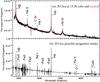 |
Fig. 1 a) Model of the spectrum of SN 2013cu at 15.5 h after the explosion (red-dashed line) and the respective observations from G14 (black). The strongest features are labeled. b) Example of a possible LBV pre-explosion spectrum of the progenitor of SN 2013cu. We note the huge difference in pre- and post-explosion morphology due to very different ionization conditions before and after the SN. |
Figure 1a shows the observed optical spectrum of 2013cu at 15.5 h after the explosion (G14) and our best-fitting CMFGEN model. We obtain that a slow, dense wind or CSM surrounds the progenitor at the time of explosion, with vwind ≲ 100 km s-1 and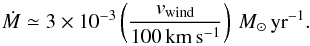 (1)We note that lower values of vwind are allowed since the narrow component of the spectral lines is unresolved by the observations. Our values of Ṁ and vwind are lower than the analytical estimates of G14 (1 × 10⁻²M⊙ yr-1 and 500 km s-1, respectively). This difference arises from our detailed line-profile modeling, which includes an accurate treatment of electron scattering. We refer the reader to Dessart et al. (2009) for a discussion on how CMFGEN treats electron scattering. Still, our determination of Ṁ/υ∞ is roughly consistent with this previous study. Our best-fitting model has LSN = 1 × 10¹⁰L⊙ and Rin = 1.5 × 1014 cm, which is consistent with the dense portions of the wind not being overrun by the SN shock front.
The early-time spectral morphology of SN 2013cu is accurately reproduced by our model (Fig. 1a). We can reproduce reasonably well the strength and shape of most features, with a narrow component and broad emission wings that are caused by electron scattering and not by the wind velocity field. The blue wings of the Balmer lines are underestimated by our models, which may be a sign that the inner wind is accelerated (Fransson et al. 2014). The strength of the He i lines is also underestimated by our models, although a larger value of Rin would reproduce the He i lines more accurately.
Our modeling allows us to directly determine the chemical composition of a SN progenitor wind. We find a significant amount of H and He, with abundances (by mass) of X ≈ 0.46± 0.2 and Y ≈ 0.52±0.2, respectively. The errors are largely dominated by the unsatisfactory fit of the He i lines, and future model improvements could possibly reduce these uncertainties significantly. We find that the wind is enhanced in N and depleted in C relative to solar values (mass fractions of 8.0×10⁻³ and 1.0 × 10⁻⁵, respectively). Assuming a solar CNO content yields a depleted O mass fraction of 1.6 × 10⁻⁴. We estimate the error in the CNO abundances to be 50%. The errors in the abundances are determined by running models with different abundances, comparing the synthetic spectra and observations by eye, and estimating the range of values that provide a satisfactory fit. Taking the errors into account, the abundances of 2013cu are consistent with having a progenitor that lost a sizable fraction of the H envelope and presents fully CNO-processed material at the surface, confirming the suggestions from G14.
Figure 2a shows the physical conditions of SN 2013cu at 15.5 h after explosion. We note that the photosphere is located in the progenitor wind. We find that the strongest lines in the 15.5 h optical spectrum, such as Hα, He ii λ5411, and N ivλ7123, are formed over an extended distance of 2−20 × 1014 cm (containing 2.2 × 10⁻²M⊙), with the bulk of the emission coming from 4−7 × 1014 cm (containing 4.5 × 10⁻³M⊙). We also obtain that the outflow is significantly ionized, with H and He being fully ionized up to large distances (≳1016 cm). The ionization structure at 15.5 h post-explosion is shown in Fig. 2b.
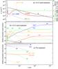 |
Fig. 2 a) Density, velocity, Rosseland optical depth, and formation regions of Hα, He ii λ5411, and N iv λ7123 (the area under the curve is proportional to the normalized equivalent width) of SN 2013cu based on our CMFGEN model at 15.5 h after the explosion. b) Predicted ionization structure at 15.5 h after the explosion. c) Predicted ionization structure of a possible LBV progenitor before the SN explosion. |
Although an apparent WN(h)-like spectrum is seen at 15.5 h after the explosion, we argue here that the spectral type of the progenitor was not the same as that seen during the post-explosion because of the very different ionization conditions at the pre- and post-explosion epochs (Fig. 2b,c). Since the number of ionizing photons at the inner boundary at 15.5 h is many orders of magnitude larger than the typical number of ionizing photons of SN progenitors, the progenitor wind is quickly ionized. Our model shows that the ionization structure after the SN explosion responds to the new SN effective temperature and huge increase in luminosity (Fig. 2b).
Because of the non-stellar origin of the apparent WN(h) post-SN explosion spectrum, we advocate here for the use of the prefix “X” (short for eXplosion) before the spectral type of such events like SN and SN impostors where a shock breakout and/or interacting CSM illuminate and ionize the precursor wind. This will avoid future confusion between spectral types seen after the explosion with those of their progenitors. Thus, in the case of the SN 2013cu spectrum at 15.5 h, the spectral type would be XWN5(h), following the WN classification scheme of Smith et al. (1996) and noting that the C iv λ5808/He ii λ5411 ratio favors the earlier classification.
3. A luminous blue variable or yellow hypergiant precursor directly before SN 2013cu
To investigate the spectral morphology of the progenitor, we compute its predicted spectrum using as input the values obtained from the post-explosion spectral modeling (Ṁ ≃ 3 × 10⁻³M⊙ yr-1, vwind ≃ 100 km s-1, and the aforementioned chemical abundances). We use CMFGEN in its standard stellar mode as described in, e.g., Groh et al. (2009), where a hydrostatic solution is computed for the subsonic region and merged with the wind solution at 0.75 of the sonic speed. The progenitor wind is assumed to accelerate following a beta-type law with β = 1. Since we have no constraints on the luminosity (L⋆) and hydrostatic radius (R⋆) of the progenitor, we assume R⋆ = 100 R⊙ and L⋆ = 5 × 10⁵L⊙ to compute its spectrum. Owing to the large Ṁ and low vwind inferred from the post-explosion spectrum, our pre-explosion models predict that the progenitor has a pseudo-photosphere with Teff ≃ 8000 K. The qualitative pre-explosion spectral morphology and Teff are only weakly dependent on L⋆ and R⋆ for sensible changes in these values, i.e., even a compact progenitor would show an LBV morphology immediately before the SN explosion. A similar situation where the hydrostatic layers are deeply buried in an optically thick wind is seen in Eta Carinae (Hillier et al. 2001, 2006; Groh et al. 2012).
Figure 1b shows a prediction of the possible pre-explosion optical spectrum. The pre- and post-explosion spectra differ significantly because of the different Teff, luminosity, and ionization structures in the two situations (Figs. 2b,c). This example of pre-explosion spectrum resembles those seen in luminous blue variables (LBVs), which are a class of unstable massive stars that are found both as a transitional stage from an O-type to a WR star (Humphreys & Davidson 1994; Groh et al. 2014) and as SN progenitors (Kotak & Vink 2006; Smith et al. 2007, 2011; Kochanek et al. 2011; Pastorello et al. 2007; Trundle et al. 2008; Gal-Yam & Leonard 2009; Groh & Vink 2011; Mauerhan et al. 2013; Ofek et al. 2013; Groh et al. 2013a,b).
Given our lack of constraints on R⋆, another possibility is that the progenitor was a cool yellow hypergiant (YHG) with Teff ≃ 5000 − 7000 K (see Groh et al. 2013b). In this case, the progenitor would be extended (R⋆> 1012 cm). The progenitor would be losing mass in an outburst similar to that of the Galactic YHG ρ Cas in the year 2000–2001 (Lobel et al. 2003), which further strengthens the link between SN 2013cu and YHGs. Of crucial importance here is that the progenitor of this SN IIb would be a YHG, and not a yellow supergiant (YSG) as often quoted in the literature (e.g., Maund et al. 2011; Van Dyk et al. 2013) because YHGs have extensive mass loss and outbursts (de Jager 1998), which is exactly what we infer for the progenitor of SN 2013cu (see discussion in Groh et al. 2013b).
While the hydrostatic radius of SN IIb progenitors have been constrained by hydrodynamical modeling of the SN lightcurve (e.g., Bersten et al. 2012), this may be challenging for SN 2013cu because of circumstellar interaction. Even then, it would be hard to differentiate between LBVs and YHGs, since they both share similar values of radii (up to several 1013 cm). To differentiate between LBVs and cool YHGs, constraints on the luminosity and/or effective temperature of the progenitor would be needed, but this is only directly accessible by detecting the progenitor in pre-explosion images. For distant events as in the case of 2013cu (d = 108 Mpc), however, this would be challenging with the current instrumentation.
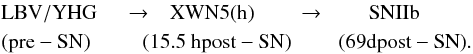
Therefore, we argue that the high value of Ṁ, relatively low vwind, and chemical abundance pattern are consistent with the progenitor being either an LBV or YHG (and not a WN star) immediately before the SN explosion. It may be possible that the star had a totally different spectral morphology before the LBV or YHG eruption phase. Based on the chemical abundances, at this pre-LBV/YHG eruptive phase, the progenitor could have been a WN, LBV, blue supergiant, YHG, or yellow supergiant, depending on its R⋆ and Ṁ. Time-dependent modeling of the SN 2013cu spectral evolution is warranted to investigate the rapid evolution before core collapse. In conclusion, we obtain the following temporal evolution for SN 2013cu and its progenitor:
4. Prospects with UV spectroscopy and outlook
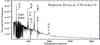 |
Fig. 3 Prediction of the early UV spectrum of SN 2013cu based on our CMFGEN model at 15.5 h after the explosion. A reddening of AV = 0.1 mag is assumed. |
The optical spectra of SN 2013cu, although it has a large wavelength coverage, is relatively poor in bright emission lines. Having access to more spectral lines would significantly aid the determination of the progenitor properties, and this would best be achieved by observing in the UV.
Ultraviolet spectroscopy offers several other advantages, such as allowing one to observe as close as possible to the peak of the spectral energy distribution of SNe at early epochs. Our predicted spectrum indicates a flux an order of magnitude higher in the UV at 15.5 h (Fig. 3). Observing in the UV allows one to probe resonance lines, such as C iv λ1548–1551, and other strong features such as He ii λ1640, and N iv λ1718. Given their high optical depths, observing UV resonance lines should provide detectable spectral features even at much lower wind densities than those of SN 2013cu. In addition, these lines allow a more precise determination of the velocity structure of the progenitor wind and SN-wind interacting region, better constraining the models. Our models predict that many Fe vi and Fe vii lines should be detectable at λλ 1200–1450. These have the potential to be used as direct probes of the progenitor and SN metallicities. We note that, in this particular case, the predicted spectrum is almost featureless in the range 2000–3000 Å, suggesting that observations should be focused below 2000 Å.
Early spectroscopy of SNe opens up a new observational window that allows the inference of progenitor properties shortly before explosion. We have shown that when these recent observations are combined with non-LTE radiative transfer modeling, quantitative information can be obtained about the progenitor, such as its chemical composition, wind velocity, and mass-loss rate. These quantities allow us to better infer the nature of the progenitor, in particular because our implementation allows the computation of a realistic progenitor spectrum, as illustrated in Fig. 1b.
In a general case, the apparent spectral morphology at early times will change according to the progenitor wind density and composition, time after SN shock breakout, and SN luminosity. We predict that this will produce a greater variety of spectral morphologies as the number of events with early-time spectra increases.
For the new events, early-time SN spectroscopy has the potential to provide even more constraints on the progenitor properties if combined with hydrodynamical modeling of the SN lightcurve and/or fortuitous pre-explosion imaging of the progenitor. Having progenitors detected in pre-explosion imaging and spectroscopically observed within a day after the SN explosion will allow us to put definitive constraints on their luminosities, effective temperatures, chemical abundances, wind velocities and mass-loss rates. This will be an important step towards a more complete understanding of the diversity of SN types and the evolutionary channels that produce their progenitors.
Acknowledgments
J.H.G. is supported by an Ambizione Fellowship of the Swiss National Science Foundation. J.H.G. thanks A. Gal-Yam, O. Yaron, and E. Ofek for making the observed spectrum of SN 2013cu available, valuable discussions, and the warm hospitality at the Weizmann Institute of Science (Israel). Discussions and comments from J. Hiller, T. Moriya, N. Smith, M. Bersten, and L. Dessart are also acknowledged, as are the comments provided by the anonymous referee.
References
- Bersten, M. C., Benvenuto, O. G., Nomoto, K., et al. 2012, ApJ, 757, 31 [NASA ADS] [CrossRef] [Google Scholar]
- Chevalier, R. A., & Fransson, C. 2006, ApJ, 651, 381 [NASA ADS] [CrossRef] [Google Scholar]
- Chevalier, R. A., & Irwin, C. M. 2011, ApJ, 729, L6 [Google Scholar]
- de Jager, C. 1998, A&ARv, 8, 145 [NASA ADS] [CrossRef] [Google Scholar]
- Dessart, L., & Hillier, D. J. 2005, A&A, 437, 667 [NASA ADS] [CrossRef] [EDP Sciences] [Google Scholar]
- Dessart, L., & Hillier, D. J. 2011, MNRAS, 410, 1739 [NASA ADS] [Google Scholar]
- Dessart, L., Hillier, D. J., Gezari, S., Basa, S., & Matheson, T. 2009, MNRAS, 394, 21 [NASA ADS] [CrossRef] [Google Scholar]
- Dessart, L., Hillier, D. J., Livne, E., et al. 2011, MNRAS, 414, 2985 [NASA ADS] [CrossRef] [Google Scholar]
- Fransson, C., Ergon, M., Challis, P. J., et al. 2014, ApJ, in press [arXiv:1312.6617] [Google Scholar]
- Gal-Yam, A., & Leonard, D. C. 2009, Nature, 458, 865 [NASA ADS] [CrossRef] [PubMed] [Google Scholar]
- Gal-Yam, A., Arcavi, I., Ofek, E. O., et al. 2014, Nature, 509, 471 [NASA ADS] [CrossRef] [Google Scholar]
- Gezari, S., Dessart, L., Basa, S., et al. 2008, ApJ, 683, L131 [NASA ADS] [CrossRef] [Google Scholar]
- Groh, J. H., & Vink, J. S. 2011, A&A, 531, L10 [NASA ADS] [CrossRef] [EDP Sciences] [Google Scholar]
- Groh, J. H., Hillier, D. J., Damineli, A., et al. 2009, ApJ, 698, 1698 [NASA ADS] [CrossRef] [Google Scholar]
- Groh, J. H., Hillier, D. J., Madura, T. I., & Weigelt, G. 2012, MNRAS, 423, 1623 [NASA ADS] [CrossRef] [Google Scholar]
- Groh, J. H., Meynet, G., & Ekström, S. 2013a, A&A, 550, L7 [NASA ADS] [CrossRef] [EDP Sciences] [Google Scholar]
- Groh, J. H., Meynet, G., Georgy, C., & Ekström, S. 2013b, A&A, 558, A131 [NASA ADS] [CrossRef] [EDP Sciences] [Google Scholar]
- Groh, J. H., Meynet, G., Ekström, S., & Georgy, C. 2014, A&A, 564, A30 [NASA ADS] [CrossRef] [EDP Sciences] [Google Scholar]
- Hillier, D. J., & Miller, D. L. 1998, ApJ, 496, 407 [NASA ADS] [CrossRef] [Google Scholar]
- Hillier, D. J., Davidson, K., Ishibashi, K., & Gull, T. 2001, ApJ, 553, 837 [NASA ADS] [CrossRef] [Google Scholar]
- Hillier, D. J., Gull, T., Nielsen, K., et al. 2006, ApJ, 642, 1098 [NASA ADS] [CrossRef] [Google Scholar]
- Humphreys, R. M., & Davidson, K. 1994, PASP, 106, 1025 [NASA ADS] [CrossRef] [Google Scholar]
- Kiewe, M., Gal-Yam, A., Arcavi, I., et al. 2012, ApJ, 744, 10 [NASA ADS] [CrossRef] [Google Scholar]
- Kochanek, C. S., Szczygiel, D. M., & Stanek, K. Z. 2011, ApJ, 737, 76 [NASA ADS] [CrossRef] [Google Scholar]
- Kotak, R., & Vink, J. S. 2006, A&A, 460, L5 [NASA ADS] [CrossRef] [EDP Sciences] [Google Scholar]
- Lobel, A., Dupree, A. K., Stefanik, R. P., et al. 2003, ApJ, 583, 923 [NASA ADS] [CrossRef] [Google Scholar]
- Mauerhan, J. C., Smith, N., Filippenko, A., et al. 2013, MNRAS, 430, 1801 [NASA ADS] [CrossRef] [Google Scholar]
- Maund, J. R., Fraser, M., Ergon, M., et al. 2011, ApJ, 739, L37 [NASA ADS] [CrossRef] [Google Scholar]
- Moriya, T. J., & Maeda, K. 2014, ApJ, 790, L16 [NASA ADS] [CrossRef] [Google Scholar]
- Moriya, T., Tominaga, N., Blinnikov, S. I., Baklanov, P. V., & Sorokina, E. I. 2011, MNRAS, 415, 199 [NASA ADS] [CrossRef] [Google Scholar]
- Moriya, T. J., Maeda, K., Taddia, F., et al. 2014, MNRAS, 439, 2917 [NASA ADS] [CrossRef] [Google Scholar]
- Nakar, E., & Sari, R. 2010, ApJ, 725, 904 [NASA ADS] [CrossRef] [Google Scholar]
- Ofek, E. O., Rabinak, I., Neill, J. D., et al. 2010, ApJ, 724, 1396 [NASA ADS] [CrossRef] [Google Scholar]
- Ofek, E. O., Sullivan, M., Cenko, S. B., et al. 2013, Nature, 494, 65 [NASA ADS] [CrossRef] [Google Scholar]
- Ofek, E. O., Sullivan, M., Shaviv, N. J., et al. 2014, ApJ, 789, 104 [NASA ADS] [CrossRef] [Google Scholar]
- Pastorello, A., Smartt, S. J., Mattila, S., et al. 2007, Nature, 447, 829 [NASA ADS] [CrossRef] [PubMed] [Google Scholar]
- Smartt, S. J. 2009, ARA&A, 47, 63 [NASA ADS] [CrossRef] [Google Scholar]
- Smith, N. 2014, ARA&A, 52, 487 [NASA ADS] [CrossRef] [MathSciNet] [Google Scholar]
- Smith, L. F., Shara, M. M., & Moffat, A. F. J. 1996, MNRAS, 281, 163 [NASA ADS] [CrossRef] [Google Scholar]
- Smith, N., Li, W., Foley, R. J., et al. 2007, ApJ, 666, 1116 [NASA ADS] [CrossRef] [Google Scholar]
- Smith, N., Li, W., Miller, A. A., et al. 2011, ApJ, 732, 63 [NASA ADS] [CrossRef] [Google Scholar]
- Soderberg, A. M., Margutti, R., Zauderer, B. A., et al. 2012, ApJ, 752, 78 [NASA ADS] [CrossRef] [Google Scholar]
- Trundle, C., Kotak, R., Vink, J. S., & Meikle, W. P. S. 2008, A&A, 483, L47 [NASA ADS] [CrossRef] [EDP Sciences] [Google Scholar]
- Van Dyk, S. D., Zheng, W., Clubb, K. I., et al. 2013, ApJ, 772, L32 [NASA ADS] [CrossRef] [Google Scholar]
All Figures
|
Fig. 1 a) Model of the spectrum of SN 2013cu at 15.5 h after the explosion (red-dashed line) and the respective observations from G14 (black). The strongest features are labeled. b) Example of a possible LBV pre-explosion spectrum of the progenitor of SN 2013cu. We note the huge difference in pre- and post-explosion morphology due to very different ionization conditions before and after the SN. |
| In the text | |
|
Fig. 2 a) Density, velocity, Rosseland optical depth, and formation regions of Hα, He ii λ5411, and N iv λ7123 (the area under the curve is proportional to the normalized equivalent width) of SN 2013cu based on our CMFGEN model at 15.5 h after the explosion. b) Predicted ionization structure at 15.5 h after the explosion. c) Predicted ionization structure of a possible LBV progenitor before the SN explosion. |
| In the text | |
|
Fig. 3 Prediction of the early UV spectrum of SN 2013cu based on our CMFGEN model at 15.5 h after the explosion. A reddening of AV = 0.1 mag is assumed. |
| In the text | |
Current usage metrics show cumulative count of Article Views (full-text article views including HTML views, PDF and ePub downloads, according to the available data) and Abstracts Views on Vision4Press platform.
Data correspond to usage on the plateform after 2015. The current usage metrics is available 48-96 hours after online publication and is updated daily on week days.
Initial download of the metrics may take a while.