| Issue |
A&A
Volume 572, December 2014
|
|
|---|---|---|
| Article Number | A115 | |
| Number of page(s) | 10 | |
| Section | Atomic, molecular, and nuclear data | |
| DOI | https://doi.org/10.1051/0004-6361/201424849 | |
| Published online | 05 December 2014 | |
R-matrix electron-impact excitation data for the Mg-like iso-electronic sequence⋆
1 Department of Physics, University of Strathclyde. Glasgow G4 0NG, UK
e-mail: luis.fernandez-menchero@strath.ac.uk
2 Department of Applied Mathematics and Theoretical Physics, University of Cambridge, Cambridge CB3 0WA, UK
Received: 22 August 2014
Accepted: 18 September 2014
Aims. Emission lines from ions in the Mg-like iso-electronic sequence can be used as reliable diagnostics of temperature and density of astrophysical and fusion plasmas over a wide range of parameters. Data in the literature are quite lacking, there are no calculations for many of the ions in the sequence.
Methods. We have carried-out intermediate coupling frame transformation R-matrix calculations which include a total of 283 fine-structure levels in both the configuration interaction target and close-coupling collision expansions. These arise from the configurations 1s2 2s2 2p6 3 {s,p,d} nl with n = 4,5, and for l = 0−4.
Results. We obtain ordinary collision strengths and Maxwell-averaged effective collision strengths for the electron-impact excitation of all the ions of the Mg-like sequence, from Al+ to Zn18 +. We compare our results with those from previous R-matrix and distorted waves calculations, where available, for some benchmark ions. We find good agreement with the results of previous calculations for the transitions n = 3−3. We also find good agreement for the most intense transitions n = 3−4. These transitions are important for populating the upper levels of the main diagnostic lines.
Key words: atomic data / techniques: spectroscopic
These data are made available in the APAP archive via http://www.apap-network.org, CHIANTI via http://www.chiantidatabase.org and open-ADAS via http://open.adas.ac.uk
© ESO, 2014
1. Introduction
Emission lines from magnesium-like ions are observed in a variety of astrophysical sources, such as the solar corona, solar transition region, stars, the interstellar medium, planetary nebulae and novae. They have been used for diagnostics of electron densities, temperatures and chemical abundances of e.g. gaseous nebulae (see, e.g. Si IIINussbaumer 1986 and Rubin et al. 1993) and the solar corona (see, e.g. Si IIIDufton et al. 1983; S VLaming et al. 1997; Fe XVDere et al. 1979). Lines from Si III were also used to suggest that non-Maxwellian electron distributions are present in the solar corona (see, e.g. Dufton et al. 1984 and Keenan et al. 1989).
Despite their importance, there is no R-matrix or distorted wave (DW) electron-impact excitation data for many ions in the sequence. Electron-impact excitation data are available for only a few of the most important ions, in most cases being calculated with small basis sets. R-matrix calculations for Al+ have been carried out by Aggarwal & Keenan (1994), with a basis set of 12 close-coupling terms, and Aggarwal (1998) with 20 levels. R-matrix calculations for Si2 + also exist: Dufton & Kingston (1989), 20 levels, and Griffin et al. (1999), 45 levels with 36 bound ones. Christensen et al. (1986) carried out distorted wave calculations for S4 +, Ar6 +, Ca8 +, Cr12 + and Ni16 + including 16 levels. Christensen et al. (1986) used the UCL-DW (Eissner 1998) code in conjunction with the JAJOM (Saraph 1972) code. S4 + electron-impact excitation data were also calculated with the R-matrix codes by Hudson & Bell (2006) on including 14 terms. Griffin et al. (1999) also carried-out 45 level R-matrix calculations for Ar6 + and Ti10 +.
Fe14 + clearly has received special attention, with several distorted wave and R-matrix calculations being performed over the years. The most recent are the distorted wave ones from Landi (2011) calculated using the Flexible Atomic Code (FAC) of Gu (2003). Landi (2011) calculated collision data from the lowest 4 levels up to 283 levels of the target. In contrast, the R-matrix calculations of Griffin et al. (1999) and Berrington et al. (2005) included just 45 levels in the close-coupling expansion, but determined collision data between all of them. Berrington et al. (2005) made a study of the inclusion of the relativistic effects in the Hamiltonian, comparing the results of Breit-Pauli and Dirac R-matrix calculations (DARC). They concluded that the difference was less than the differences which could be expected due to uncertainties in the atomic structure.
Electron-impact excitation data for Ni16 + have been calculated by Bhatia & Landi (2011), using the FAC distorted wave code, from the lowest 4 levels up to the 159 levels of their target expansion, and by Hudson et al. (2009, 2012) using the Dirac R-matrix suite of codes on including 37 close-coupling levels.
We did not find any atomic collision data in the literature for the rest of the ions in the sequence which we consider here also: P3 +, Cl5 +, K7 +, Sc9 +, V11 +, Mn13 +, Co15 +, Cu17 + and Zn18 +.
In present work we carry-out an intermediate coupling frame transformation (ICFT) R-matrix calculation including a total of 283 levels in both the configuration interaction (CI) and the close-coupling expansions. This is the same target basis as used by Landi (2011), but of course we consider all inelastic transitions. Cascading effects following collisional excitation up to the n = 5 shell can be examined within models using this basis set expansion. We use the same basis set and method for the whole iso-electronic sequence, from Al+ up to Zn18 +. The present data therefore includes significantly more transitions than the previous published works for Mg-like ions, where they exist.
Because of its diagnostic importance, the discussion of the target for Si2+ deserved special attention. One of the main diagnostic lines turns out to have a strongly-mixed upper level (see below), so we validated our target for this ion with several structure calculations and comparisons with previous calculations and observations. Details are presented in Del Zanna et al. (2014).
The paper is organised as follows. In Sect. 2 we give details of our description of the atomic structure and in Sect. 3 that of the R-matrix calculation. In Sect. 4 we show some representative results and compare them with the results of other R-matrix calculations and with distorted wave ones. The main conclusions are presented in Sect. 5. Atomic units are used unless otherwise specified. The atomic data are made available at our APAP network web page1. They will also be uploaded online in the CHIANTI atomic database2 (Landi et al. 2013) and the Atomic Data and Analysis Structure (open-ADAS3). This work is part of the UK APAP Network and is complementary to our previous work on other sequences. The most recent work was on the boron-like (Liang et al. 2012) and beryllium-like (Fernández-Menchero et al. 2014).
2. Structure
To obtain the wave functions of the isolated target we used the autostructure program (Badnell 2011), the approach is the same as that described in our previous work (Fernández-Menchero et al. 2014) but utilizing a different set of configurations. autostructure carries-out a diagonalization of the Breit–Pauli Hamiltonian (Eissner et al. 1974) to obtain the eigen states and energies of the target. Relativistic terms, viz. mass-velocity, spin-orbit, and Darwin, are included as a perturbation. We describe the multi-electron electrostatic interactions using a Thomas-Fermi-Dirac-Amaldi model potential with scaling parameters λnl. We determine the λnl through a variational method in which we minimize the equally-weighted sum of the energies of all the terms. We included a total of 15 atomic orbitals in the basis set: 1s, 2s, 2p, 3s, 3p, 3d, 4s, 4p, 4d, 4f, 5s, 5p, 5d, 5f, 5g. In the configuration interaction we included all the configurations { (1s2 2s2 2p6)3s2, 3s 3p, 3s 3d, 3p2, 3p 3d, 3d2, 3s nl, 3p nl, 3d nl }, for all nl orbitals previously mentioned with n ≥ 4, for a total of 33 configurations. The minimized values of the scaling parameters are shown in Table 2 for all the ions in the sequence.
For the configuration list detailed above, we obtain 149 LS terms, which on recoupling to take account of the spin-orbit interaction, give rise to 283 levels. The intermediate coupling (IC) energies obtained for the target levels of three sample ions: S4 +, Ar6 + and Fe14 +, are shown in Tables 3−5 respectively. The level energies are compared with the observed ones taken from the tables of the National Institute of Standards and Technology (NIST4) database: Martin et al. (1990) for sulphur, Saloman (2010) for argon, and Sugar & Corliss (1985) and Shirai et al. (2000) for iron; and with the previous theoretical calculations collected in the CHIANTI database: Christensen et al. (1986) for sulphur and argon, and Landi (2011) for iron. The agreement of the present energies with the observed values is within 1.5%, with a few exceptions in the lower excited singlet levels, and the relative errors are smaller in the present work than in previous theoretical ones with smaller basis sets, and more or less equal to the ones of Landi (2011) with the same configuration set. The energy values for the rest of the levels and the other ions of the sequence not shown in Tables 3−5 can be found online in CHIANTI5 and open-ADAS6 databases.
To check the quality of the calculated wave functions of the target we compare the oscillator strengths (gf values) for selected transitions in Table 1 for Fe14 + with data from Landi (2011), which can be found on line in the CHIANTI database. Very good agreement, within 5%, is found in general.
Comparison of gf values for some selected transitions of the ion Fe14 +. L11: Landi (2011). A (B) denotes A × 10B.
Thomas-Fermi-Dirac-Amaldi potential scaling parameters used for the autostructure calculations.
S4 + target levels.
Ar6 + target levels.
Fe14 + target levels.
As a further check of our atomic structure, we show in Fig. 1 a global comparison our oscillator strengths (gf values) with the results of Christensen et al. (1986) for sulphur, and of Landi (2011) for iron. We plot in the x-axis the results of present work, and in the y-axis the comparative ones, so points lying on the diagonal x = y mean complete agreement between the two sets. Practically all the oscillator strengths for transitions (from all lower levels) to the upper n = 4 levels lie on the diagonal x = y, with deviations smaller than 2% for both ions. For transitions up to n = 5 in Fe14 + the main body of the points lies on the diagonal also. The points which are spread far from the diagonal (about 100 of the total 1200 shown) correspond to transitions with levels with configurations 5f and 5g, the last orbitals included in our basis. As they are the last bound levels, the description of these excited levels can vary with respect to the previous works since there are no configurations which lie above to “correct” them via CI. This is the likely reason for the differences in the gf values for these transitions. For S4 +, the work of Christensen et al. (1986) just shows 22 transitions k − k′, with k = 1 − 5 and k′ = 1 − 16 levels. The agreement between Christensen et al. (1986) results and ours is better than 5%.
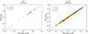 |
Fig. 1 Comparative plot of oscillator strengths for S4 + and Fe22 +. x axis: present work; y axis: S4 + (Christensen et al. 1986); Fe14 + (Landi 2011). These are denoted by: ° for n = 3 upper levels; □ for n = 4 upper levels; × for n = 5 upper levels. |
In the particular case of Si2 +, the 3s3p 1P1 − 3s4s 1S0 transition was used to suggest that non-Maxwellian electron distributions are present in the solar corona (see, e.g. Dufton et al. 1984 and Keenan et al. 1989). It turns out that the upper level 3s4s 1S0 is strongly LS-mixed with the 3p21S0. The energy difference between these two levels is only 5625 cm-1. During the optimization process of the scaling parameters of this ion we had to be careful to get the correct mixing between these two levels. The A-values for the decays from these levels are very sensitive to the structure. The scaling parameters which lead to the optimum value of the Einstein coefficient for that transition are the ones shown in Table 2. We refer to Del Zanna et al. (2014) for a more detailed description of this specific ion, comparisons with previous calculations and with observations.
3. Scattering
For the scattering calculation, we used the same approach as in our previous work (Fernández-Menchero et al. 2014), which consists of an R-matrix formalism (Hummer et al. 1993; Berrington et al. 1995) combined with an intermediate coupling frame transformation (Badnell & Griffin 2001; Badnell et al. 2001) to include the spin-orbit mixing efficiently and accurately.
The calculation in the inner region of the R-matrix method was split into two parts, one including electron exchange effects and a second one using a non-exchange approximation.
The exchange calculation included angular momenta up to 2J = 30, and the non exchange extended up to 2J = 80. For higher angular momenta up to infinity, we used the top-up formula of the Burgess sum rule (Burgess 1974) for dipole allowed transitions, and a geometric series for the remaining non-forbidden transitions, i.e. those with a non-zero infinite energy Born limit (Badnell & Griffin 2001).
The R-matrix outer region calculation was also split into two parts. For the resonance region, where impact energies are below the excitation energy of the last calculated level, a fine energy mesh was applied in order to resolve the resonances. For energies above the last energy threshold a coarse mesh was used to resolve the smooth background. This coarse mesh was around 10-4z2 Ry, with z the ion charge Z − 12, Z being the atomic number.
In the resonance region, we have the difficulty that the characteristic scattering energy increases as a factor z2 with the charge of the ion, nevertheless the width of the resonances remains constant. If we attempt to resolve the resonances to the same degree along the whole sequence we have then to reduce the energy step of the fine mesh by a factor z2 too. This number of points becomes computationally unreasonable for the highest few charge states in the sequence. We used the same practical criterion as in Witthoeft et al. (2007) and we increased the number of grid points by a factor z; this samples and converges the resonance structure satisfactorily. Thus, we use a fine energy mesh step which varies continuously versus the ionic charge, from 1.4 × 10⁻⁴ for Al+ up to 3.6 × 10⁻⁶ for Zn18 +.
We obtain the Maxwell-averaged effective collision strengths for electron-impact excitation, Υ(i − j), on performing a convolution of the ordinary collision strengths, Ω, with a Maxwellian velocity distribution for the electrons:  (1)where u = E/kT, E is the final energy of the scattered electron, T the electron temperature and k the Boltzmann constant. We calculated the effective collision strengths for a wide range of temperatures, from ~z2 × 102 to ~z2 × 105 K, which covers the temprature range of interest for each ion for both astrophysical and fusion plasmas.
Nevertheless, in some radiating astrophysical sources the electron velocity distribution differs from a Maxwellian one, e.g. the solar wind (Bryant 1996). As such, the study of non-Maxwellian velocity distributions has become more intensive in recent years, see for example Dudìk et al. (2014a,b); Storey & Sochi (2013); Dzifčáková & Dudík (2013). In models with enhanced high-energy tails, the kinetic energy of the electrons typically follows a κ distribution:  (2)where κ parameterizes the family, Eκ is the characteristic energy such that κEκ/ (κ − 3/2) = kTeff, where Teff is the effective temperature, i.e.
  ,
,  being the mean electron energy. The κ distribution tends to a Maxwellian one as κ tends to infinity.
In the Maxwellian case, the effective collision strengths for de-excitation, Υ(i − j), are equal to the ones for excitation. In the case of a non-Maxwellian distribution this is no longer true. The de-excitation effective collision strength is given by (1), but with the Maxwellian distribution replaced by the kappa one (2). The excitation effective collision strength expression involves additional factors of the excitation energy, see e.g. Bryans (2005) for specific details.
To converge the convolution integrals at high temperatures, one has to extend the calculated ordinary collision strengths to higher collision energies, it being impractical, and unnecessary, to do so explicitly using the R-matrix method. Instead, we calculate the infinite-energy Born and radiative dipole limits with autostructure, depending on the transition type. Once these limits are calculated we interpolate in the Burgess–Tully scaled domain (Burgess & Tully 1992) for each specific transition type.
For Maxwellian distributions, which is the main goal of present work, we store online the effective collision strengths as a type 3 ADAS Atomic Data Format adf04 file in the open-ADAS database. For the use of non-Maxwellian distributions it is necessary to make the original ordinary collision strengths Ω available, so that they can be convoluted by any kind of energy distribution. R-matrix calculations with a few hundred levels and ~104 energies, such as those performed here, easily generate (compressed) Gbtye sized files. These are impractical to webserve. To this end, we have implemented an energy-averaging of the ordinary collision strengths using a quasi-logarithmic energy mesh for the final scattered electron energy. The representation in terms of the final scattered energy maintains resolution for transitions between excited states which is lost if, as is typically done, the initial incident energy is used. The binned collision strengths (at typically 100–200 energies) are stored as a (type 5) ADAS Atomic Data Format adf04 file, which compress to a few Mbytes.
4. Results
We calculated the ordinary collision strengths and Maxwell-averaged effective collision strengths for the electron-impact excitation of all ions in the Mg-like iso-electronic sequence, from Al+ to Zn18 +, for all transitions between the 283 close-coupling fine-structure levels, which gives rise to a total of 39 903 inelastic transitions for each ion.
The effective collision strengths have been stored as a (type 3) ADAS adf04 file. These files also contain the full set of A-values up to E3/M2 as calculated by autostructure using the structure described in Sect. 2. These data can be used for the spectroscopic diagnostic determination of the temperature and density of astrophysical and fusion plasmas.
As a sample of the results, we show in Fig. 2 the collision strengths for some important transitions within the n = 3 complex for the benchmark ions in the Mg-like sequence. We compare with previous distorted wave calculations of Christensen et al. (1986) for sulphur and argon, and Landi (2011) for iron. We have also performed a distorted wave calculation, using the same atomic structure as used for the R-matrix one. We show results for four different types of transitions: dipole allowed (1 − 5), dipole allowed through spin-orbit mixing (1 − 3), a double electron jump Born transition (1 − 7), and a forbidden one (1 − 10). Above the resonance region, the collision strength for dipole allowed transitions diverges logarithmically as the energy tends to infinity, while for non-dipole allowed transitions it tends to a constant and for forbidden transitions the collision strength tends to zero as E-2 in the infinite energy limit.
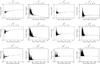 |
Fig. 2 Electron-impact excitation collision strengths versus the impact energy for some selected transitions within the n = 3 complex. Full line: present work; ×: distorted wave calculation with present structure; □: distorted wave calculations of Christensen et al. (1986) for S4 + and Ar6 +, and Landi (2011) for Fe14 +; ⋄: distorted wave calculation of Christensen et al. (1985) for Fe14 +. |
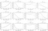 |
Fig. 3 Electron-impact excitation effective collision strengths versus the electron temperature for some selected transitions within the n = 3 complex. Full line: present calculation; dashed line: results tabulated in the CHIANTI data base, S4 + and Ar6 +Christensen et al. (1986), Fe14 +Berrington et al. (2005). |
Figure 3 shows the Maxwell-averaged effective collision strengths for the same transitions. The figure also shows a comparison with previous calculations: Christensen et al. (1986) for S4 + and Ar6 +, and Berrington et al. (2005) for Fe14 +.
At low temperatures the centre of the Maxwellian envelope overlies the resonance region, so at these temperatures the effective collision strength is quite sensitive to the resolution of the resonances. Thus, we have carried-out a convergence study to check that we used a fine enough electron energy mesh for the ions under consideration. The final mesh chosen was detailed in Sect. 3. The differences found with the distorted wave results of Christensen et al. (1986) and Landi (2011) at low temperatures are caused by the lack of resonance structure in the distorted wave calculations. At high temperatures, the agreement between the R-matrix and distorted waves results is quite good. The transition (1 − 3) shows an interesting z-dependence – spin-orbit mixing becoming increasingly important as the charge increases. For sulphur, this transition behaves as a forbidden one at temperatures of physical interest, but for iron it shows dipole-like behaviour.
The collision strengths for the Fe14 +1 − 10 (J = 0 − J′ = 0) transition as calculated with the R-matrix codes are up to a factor 12 − 18 larger than the ones obtained with the distorted wave approximation. Our distorted wave collision strengths, calculated with the same structure as with the R-matrix codes, agree with the distorted wave results of Landi (2011). They hardly change if we use instead the atomic structure of Christensen et al. (1985). So the discrepancies do not lie in the atomic structure but in the differences between the scattering methods. Looking at the same transition for the other ions shown, S4 + and Ar6 +, the differences between the results calculated with R-matrix and distorted wave remain. Note that in the plots for this transition in Fig. 2, for S4 + (actually, 1 − 13 then) and Ar6 +, the present distorted wave results (symbol ×) are off the bottom of the scale. The discrepancy remains and so these differences are not related to the spin-orbit interaction.
In the Burgess-Tully (Burgess & Tully 1992) reduced plots for transition 1 − 10 of Fe14 + of Fig. 4, the results of all calculations tend approximately to the same infinite energy limit point. We note that the results of Christensen et al. (1985) were calculated with the UCL-DW and JAJOM codes. These codes have the capability to convert the full K-matrix for the 16 levels to the T/S-matrices in a unitarized fashion. Both AS-DW and FAC use a two-state (initial-plus-final) conversion. The former has long been known to take account of a degree of coupling within the distorted wave formalism (e.g. Burgess et al. 1970). This is a possible explanation for the differences between the distorted wave results for this very weak transition.
The most probable decay of level 10 (3p21S0) is the E1 transition to level 5 ( ), with a wavelength of 325.0 Å. The 1 − 10 transition is a one-photon forbidden one, two electron jump, and the collision strength is small, so significant population of level 10 will come from cascading form higher levels. The CHIANTI atomic model, which uses the Berrington et al. (2005)R-matrix excitation data, predicts that about 64% of the population of this level is due to direct excitation from the ground state, and about 32% comes from cascading from the 3p3d 1P1 (level 26), which in turn is populated by direct excitation from the ground state by about 45%.
The intensity of the 5 − 10 transition is therefore partly affected by the 1 − 10 excitation. It is interesting to note that the CHIANTI atomic model predicts an intensity for the 5 − 10325.0 Å line that is about 50% stronger than what is observed in solar active region high-resolution SERTS-97 spectra by Brosius et al. (2000). Therefore, the Berrington et al. (2005) collision strengths clearly overestimate the collision strength from the ground. Indeed our calculations predict significantly lower collision strengths than Berrington et al. (2005) for this transition (1 − 10, bottom right plot in Fig. 3).
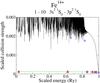 |
Fig. 4 Burgess-Tully scaled electron-impact excitation collision strengths for the transition 1 − 10: 3s21S0 − 3p21S0 in Fe14 +. Full line: present R-matrix work; ×: distorted wave calculation with the present structure; □: distorted wave calculation of Landi (2011); ⋄: distorted wave calculation of Christensen et al. (1985); △: distorted wave calculations with autostructure and the atomic structure of Christensen et al. (1985). |
As a sample of our results, we show a set of non-Maxwellian effective collision strengths for some transitions which are interesting for astrophysics. In the solar transition region the Si2 + ion has a maximum in the abundance fraction (T ≈ 5 × 10⁴ K), and therefore transitions may be susceptible to non-Maxwellian distributions, for example direct excitations from the ground state to other singlets, e.g. 3p21D2, 3p21S0 or 3s4s 1S0, amongst others.
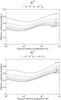 |
Fig. 5 Electron-impact de-excitation effective collision strengths versus effective electron temperature for selected transitions in Si2 +. The values of κ used for the electron velocity distribution are shown on the curves: κ =2.0, 2.5, 3.0, 4.0, 6.0, 10.0 and ∞ in decreasing order of the effective collision strength. |
In Fig. 5 we show the effective collision strengths for Si2+ transitions present in solar transition region which can be affected by a non-Maxwellian distribution. These transitions are forbidden ones so their collision strengths Ω fall-off rapidly (as E-2) at high collision energies. Thus, upon averaging, the effective collision strengths are sensitive to any deviation of the high energy tail of the velocity distribution from Maxwellian. This is normally represented by a κ distribution. We show results for several values of κ, converging on the Maxwellian.
5. Conclusions
We have presented a complete data set of ICFT R-Matrix calculations for the electron-impact excitation of all ions in the Mg-like iso-electronic sequence from Al+ to Zn18 +. We have shown a selected set of collision strengths and effective collision strengths for some important n = 3 transitions and ions and find good agreement with previous similar calculations, where they exist. Significant discrepancies with earlier distorted wave calculations are found. We have also presented some effective collision strengths assuming non-Maxwellian velocity distributions for the colliding electrons.
The present atomic data are a significant extension and improvement over previous ones, and are the first ones for many ions in the Mg-like sequence. With our basis set, the modelling of emission lines can now include cascading effects from levels up to n = 5. With the present data, emission lines from Mg-like ions can reliably be used for diagnostics of temperature and density of astrophysical and fusion plasmas.
Work is in progress to apply the same type of calculations to other iso-electronic sequences. We are carrying out calculations for the C-like, N-like and O-like sequences. Together with our previous calculations for the F-like Witthoeft et al. (2007), Ne-like Liang & Badnell (2010), Li-like Liang & Badnell (2011), Be-like Fernández-Menchero et al. (2014) and B-like Liang et al. (2009), the whole of the L-shell of iso-electronic sequences will be completed.
Acknowledgments
The present work was funded by STFC (UK) through the University of Strathclyde UK APAP network grant ST/J000892/1 and the University of Cambridge DAMTP astrophysics grant.
References
- Aggarwal, K. M. 1998, ApJSS, 118, 589 [NASA ADS] [CrossRef] [Google Scholar]
- Aggarwal, K. M., & Keenan, F. P. 1994, J. Phys. B, 27, 5321 [NASA ADS] [CrossRef] [Google Scholar]
- Badnell, N. R. 2011, Comput. Phys. Commun., 182, 1528 [NASA ADS] [CrossRef] [Google Scholar]
- Badnell, N. R., & Griffin, D. C. 2001, J. Phys. B, 34, 681 [Google Scholar]
- Badnell, N. R., Griffin, D. C., & Mitnik, D. M. 2001, J. Phys. B: Atom., Mol. Opt. Phys., 34, 5071 [Google Scholar]
- Berrington, K. A., Eissner, W. B., & Norrington, P. H. 1995, Comput. Phys. Commun., 92, 290 [NASA ADS] [CrossRef] [Google Scholar]
- Berrington, K. A., Ballance, C. P., Griffin, D. C., & Badnell, N. R. 2005, J. Phys. B: Atom., Mol. Opt. Phys., 38, 1667 [NASA ADS] [CrossRef] [Google Scholar]
- Bhatia, A. K., & Landi, E. 2011, At. Data Nucl. Data Tables, 97, 189 [NASA ADS] [CrossRef] [Google Scholar]
- Brosius, J. W., Thomas, R. J., Davila, J. M., & Landi, E. 2000, ApJ, 543, 1016 [NASA ADS] [CrossRef] [Google Scholar]
- Bryans, P. 2005, Ph.D. Thesis, University of Strathclyde [Google Scholar]
- Bryant, D. A. 1996, J. Plasma Phys., 56, 87 [NASA ADS] [CrossRef] [Google Scholar]
- Burgess, A. 1974, J. Phys. B: Atom. Mol. Phys., 7, L364 [Google Scholar]
- Burgess, A., & Tully, J. A. 1992, A&A, 254, 436 [NASA ADS] [Google Scholar]
- Burgess, A., Hummer, D. G., & Tully, J. A. 1970, Philos. Trans. R. Soc. London, Ser. A, 266, 225 [Google Scholar]
- Christensen, R. B., Norcross, D. W., & Pradhan, A. K. 1985, Phys. Rev. A, 32, 93 [NASA ADS] [CrossRef] [Google Scholar]
- Christensen, R. B., Norcross, D. W., & Pradhan, A. K. 1986, Phys. Rev. A, 34, 4704 [NASA ADS] [CrossRef] [Google Scholar]
- Del Zanna, G., Fernández-Menchero, L., & Badnell, N. R. 2014, A&A, in press, DOI: 10.1051/0004-6361/201424394 [Google Scholar]
- Dere, K. P., Widing, K. G., Mason, H. E., & Bhatia, A. K. 1979, ApJSS, 40, 341 [NASA ADS] [CrossRef] [Google Scholar]
- Dudìk, J., Zanna, G. D., Dzifčáková, E., Mason, H. E., & Golub, L. 2014a, ApJ, 780, L12 [NASA ADS] [CrossRef] [Google Scholar]
- Dudìk, J., Zanna, G. D., Mason, H. E., & Dzifčáková, E. 2014b, A&A, 570, A124 [NASA ADS] [CrossRef] [EDP Sciences] [Google Scholar]
- Dufton, P. L., & Kingston, A. E. 1989, MNRAS, 241, 209 [NASA ADS] [CrossRef] [Google Scholar]
- Dufton, P. L., Kingston, A. E., & Scott, N. S. 1983, J. Phys. B., 16, 3053 [Google Scholar]
- Dufton, P. L., Kingston, A. E., & Keenan, F. P. 1984, ApJ., 280, L35 [NASA ADS] [CrossRef] [Google Scholar]
- Dzifčáková, E., & Dudík, J. 2013, ApJSS, 206, 6 [NASA ADS] [CrossRef] [Google Scholar]
- Eissner, W. 1998, Comput. Phys. Commun., 114, 295 [NASA ADS] [CrossRef] [Google Scholar]
- Eissner, W. M., Jones, M., & H, N. 1974, Comput. Phys. Commun., 8, 270 [NASA ADS] [CrossRef] [Google Scholar]
- Fernández-Menchero, L., Zanna, G. D., & Badnell, N. R. 2014, A&A, 566, A104 [NASA ADS] [CrossRef] [EDP Sciences] [Google Scholar]
- Griffin, D. C., Badnell, N. R., Pindzola, M. S., & Shaw, J. A. 1999, J. Phys. B, 32, 2139 [NASA ADS] [CrossRef] [Google Scholar]
- Gu, M. F. 2003, ApJ., 590, 1131 [NASA ADS] [CrossRef] [Google Scholar]
- Hudson, C. E., & Bell, K. L. 2006, A&A, 452, 1113 [NASA ADS] [CrossRef] [EDP Sciences] [Google Scholar]
- Hudson, C. E., Norrington, P. H., & Ramsbottom, C. A. 2009, J. Phys. Conf. Ser., 163, 012060 [NASA ADS] [CrossRef] [Google Scholar]
- Hudson, C. E., Norrington, P. H., Ramsbottom, C. A., & Scott, M. P. 2012, A&A, 537, A12 [NASA ADS] [CrossRef] [EDP Sciences] [Google Scholar]
- Hummer, D. G., Berrington, K. A., Eissner, W., et al. 1993, A&A, 279, 298 [NASA ADS] [Google Scholar]
- Keenan, F. P., Dufton, P. L., Kingston, A. E., & Cook, J. W. 1989, ApJ, 340, 1135 [NASA ADS] [CrossRef] [Google Scholar]
- Laming, J. M., Feldman, U., Schühle, U., et al. 1997, ApJ, 485, 911 [NASA ADS] [CrossRef] [Google Scholar]
- Landi, E. 2011, At. Data Nucl. Data Tables, 97, 587 [NASA ADS] [CrossRef] [Google Scholar]
- Landi, E., Young, P. R., Dere, K. P., Zanna, G. D., & Mason, H. E. 2013, ApJ, 763, 86 [NASA ADS] [CrossRef] [Google Scholar]
- Liang, G. Y., & Badnell, N. R. 2010, A&A, 518, A64 [NASA ADS] [CrossRef] [EDP Sciences] [Google Scholar]
- Liang, G. Y., & Badnell, N. R. 2011, A&A, 528, A69 [NASA ADS] [CrossRef] [EDP Sciences] [Google Scholar]
- Liang, G. Y., Whiteford, A. D., & Badnell, N. R. 2009, A&A, 499, 943 [NASA ADS] [CrossRef] [EDP Sciences] [Google Scholar]
- Liang, G. Y., Badnell, N. R., & Zhao, G. 2012, A&A, 547, A87 [NASA ADS] [CrossRef] [EDP Sciences] [Google Scholar]
- Martin, W. C., Zalubas, R., & Musgrove, A. 1990, J. Phys. Chem. Ref. Data, 19, 821 [NASA ADS] [CrossRef] [Google Scholar]
- Martin, W. C., Sugar, J., Musgrove, A., & Dalton, G. R. 1995, NIST Database for Atomic Spectroscopy, Version 1.0, NIST Standard Reference Data base 61 [Google Scholar]
- Nussbaumer, H. 1986, A&A, 155, 205 [NASA ADS] [Google Scholar]
- Rubin, R. H., Dufour, R. J., & Walter, D. K. 1993, ApJ, 413, 242 [NASA ADS] [CrossRef] [Google Scholar]
- Saloman, E. B. 2010, J. Phys. Chem. Ref. Data, 39, 033101 [NASA ADS] [CrossRef] [Google Scholar]
- Saraph, H. E. 1972, A&A, 3, 256 [Google Scholar]
- Shirai, T., Sugar, J., Musgrove, A., & Wiese, W. L. 2000, J. Phys. Chem. Ref. Data, Monograph N 8 [Google Scholar]
- Storey, P. J., & Sochi, T. 2013, MNRAS, 430, 599 [NASA ADS] [CrossRef] [Google Scholar]
- Sugar, J., & Corliss, C. 1985, J. Phys. Chem. Ref. Data, 1 [Google Scholar]
- Witthoeft, M. C., Whiteford, A. D., & Badnell, N. R. 2007, J. Phys. B: At. Mol. Opt. Phys., 40, 2969 [Google Scholar]
All Tables
Comparison of gf values for some selected transitions of the ion Fe14 +. L11: Landi (2011). A (B) denotes A × 10B.
Thomas-Fermi-Dirac-Amaldi potential scaling parameters used for the autostructure calculations.
All Figures
|
Fig. 1 Comparative plot of oscillator strengths for S4 + and Fe22 +. x axis: present work; y axis: S4 + (Christensen et al. 1986); Fe14 + (Landi 2011). These are denoted by: ° for n = 3 upper levels; □ for n = 4 upper levels; × for n = 5 upper levels. |
| In the text | |
|
Fig. 2 Electron-impact excitation collision strengths versus the impact energy for some selected transitions within the n = 3 complex. Full line: present work; ×: distorted wave calculation with present structure; □: distorted wave calculations of Christensen et al. (1986) for S4 + and Ar6 +, and Landi (2011) for Fe14 +; ⋄: distorted wave calculation of Christensen et al. (1985) for Fe14 +. |
| In the text | |
|
Fig. 3 Electron-impact excitation effective collision strengths versus the electron temperature for some selected transitions within the n = 3 complex. Full line: present calculation; dashed line: results tabulated in the CHIANTI data base, S4 + and Ar6 +Christensen et al. (1986), Fe14 +Berrington et al. (2005). |
| In the text | |
|
Fig. 4 Burgess-Tully scaled electron-impact excitation collision strengths for the transition 1 − 10: 3s21S0 − 3p21S0 in Fe14 +. Full line: present R-matrix work; ×: distorted wave calculation with the present structure; □: distorted wave calculation of Landi (2011); ⋄: distorted wave calculation of Christensen et al. (1985); △: distorted wave calculations with autostructure and the atomic structure of Christensen et al. (1985). |
| In the text | |
|
Fig. 5 Electron-impact de-excitation effective collision strengths versus effective electron temperature for selected transitions in Si2 +. The values of κ used for the electron velocity distribution are shown on the curves: κ =2.0, 2.5, 3.0, 4.0, 6.0, 10.0 and ∞ in decreasing order of the effective collision strength. |
| In the text | |
Current usage metrics show cumulative count of Article Views (full-text article views including HTML views, PDF and ePub downloads, according to the available data) and Abstracts Views on Vision4Press platform.
Data correspond to usage on the plateform after 2015. The current usage metrics is available 48-96 hours after online publication and is updated daily on week days.
Initial download of the metrics may take a while.