| Issue |
A&A
Volume 570, October 2014
|
|
|---|---|---|
| Article Number | A56 | |
| Number of page(s) | 9 | |
| Section | Atomic, molecular, and nuclear data | |
| DOI | https://doi.org/10.1051/0004-6361/201424508 | |
| Published online | 16 October 2014 | |
Atomic data for astrophysics: improved collision strengths for Fe viii⋆
1
DAMTP, Centre for Mathematical Sciences,
Wilberforce road Cambridge,
CB3 0WA,
UK
e-mail:
g.del-zanna@damtp.cam.ac.uk
2
Department of Physics, University of Strathclyde,
Glasgow, G4 0NG, UK
Received: 1 July 2014
Accepted: 12 August 2014
We describe, and present the results of, a new large-scale R-matrix scattering calculation for the electron collisional excitation of Fe viii. We first discuss the limitations of the previous calculations, in particular concerning some strong EUV lines observed in the solar corona by the Hinode EUV Imaging Spectrometer. We then present a new target which represents an improvement over the previous ones for this particularly complex ion. We developed a new method, based on the use of term energy corrections within the intermediate coupling frame transformation method, to calculate the collision strengths. We compare predicted and observed line intensities using laboratory and solar spectra, finding excellent agreement for all the main soft X-ray and extreme ultraviolet (EUV) transitions, using the present atomic data. In particular, we show that Fe viii EUV lines observed by Hinode EIS can now be used to provide reliable electron temperatures for the solar corona.
Key words: atomic data / line: identification / techniques: spectroscopic
The full dataset (energies, transition probabilities and rates) is only available in electronic form at our APAP website (http://www.apap-network.org) as well as at the CDS via anonymous ftp to cdsarc.u-strasbg.fr (130.79.128.5) or via http://cdsarc.u-strasbg.fr/viz-bin/qcat?J/A+A/570/A56
© ESO, 2014
1. Introduction
Fe viii lines are prominent in EUV/UV solar observations, in particular those from the Hinode EUV Imaging Spectrometer (EIS, see Culhane et al. 2007), as discussed in Young et al. (2007); Del Zanna (2009b); Young & Landi (2009). As discussed in Del Zanna (2009b), the Hinode EIS Fe viii lines can in principle be used to measure electron temperatures for active region loops. However, significant discrepancies between observed and predicted line intensities were found, as described in Del Zanna (2009b; one of the series where atomic data are benchmarked against astrophysical and laboratory data, see Del Zanna et al. 2004).
The collisional data used in Del Zanna (2009b) were those of Griffin et al. (2000). Their scattering target included only 33 LS terms from the seven configurations: 3s2 3p6 3d, 3s2 3p5 3d2, 3s2 3p5 3d 4s, 3s2 3p6 4s, 3s2 3p6 4p, 3s2 3p6 4d, and 3s2 3p6 4f. As already pointed out by Griffin et al. (2000), this target is not very accurate for several important transitions now observed by Hinode EIS, since larger CI structure calculations showed variations of the order of 30% in their radiative rates. To build their larger CI structure calculations, Griffin et al. (2000) included terms from the 3s2 3p4 3d3, 3s2 3p3 3d4, and 3s2 3p4 3d2 4f configurations, which mix strongly with the 3s2 3p6 3d, 3s2 3p5 3d2, and 3s2 3p6 4f.
Obtaining an accurate structure for this ion is challenging, as shown by Zeng et al. (2003), where several large-scale multi-configuration Hartree-Fock (MCHF) calculations were carried out. The importance of including core-valence electron correlations was highlighted there. The authors reached convergence in the values of the oscillator strengths for the main transitions with their case D (which included correlations of the type 3p3 −3d3). However, their level energies were not very accurate. Also, and more importantly, they did not include in the structure calculations the 3s2 3p6 4p, which mixes strongly with the 3s2 3p5 3d2, and produces some of the strongest EUV lines for this ion.
In our previous study (Del Zanna 2009b), we found a “benchmark” configuration basis, comprising of 23 configurations and n = 5 correlation orbitals, that produced reasonably accurate energies for the n = 3 levels. To further improve the energies, term energy corrections were also applied. As we discussed in Del Zanna (2009b), it is difficult to obtain accurate energies for several levels, in particular: a) the 3s2 3p5 3d22P3/2 which mixes strongly with 3s2 3p6 4p 2P3/2 and 3s2 3p5 3d22P3/2; b) 3s2 3p6 4p 2P3/2; c) 3s2 3p5 3d22P1/2 which mixes strongly with the 3s2 3p5 3d22P1/2 and 3s2 3p5 3d22P1/2. We used this benchmark configuration basis to adjust the Griffin et al. collision strengths of the dipole-allowed transitions. We then showed that the model ion obtained in this way improves the comparison with observed line intensities. However, significant discrepancies were still present, in particular for the important 3s2 3p5 3d24D levels, which we identified and showed that are a potentially useful temperature diagnostic.
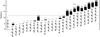 |
Fig. 1 Term energies of the target levels (25 configurations). The lowest 209 terms which produce levels having energies below the dashed line have been retained for the close-coupling expansion. |
Tayal & Zatsarinny (2011) recently carried out a large-scale atomic calculation for Fe viii. The scattering target was much larger than the one adopted by Griffin et al. It included the 3s2 3p6 3d, 3s2 3p5 3d2, 3s2 3p6 4l (l = s, p, d, f), 3s 3p6 3d2, 3s2 3p6 5l (l = s, p, d, f, g), and 3s2 3p5 3d 4s configurations, for a total of 108 fine-structure levels. Tayal & Zatsarinny (2011) justified the accuracy of the target by showing a comparison between theoretical and experimental level energies, and between the length and velocity forms of the oscillator strengths. It is indeed true (see below for a detailed comparison) that energies are closer to the experimental ones, compared to previous calculations. However, close inspection of Table 4 in Tayal & Zatsarinny (2011) shows that their oscillator strengths for a few transitions are significantly different than those of the large structure calculations (Zeng et al. 2003; Del Zanna 2009b), in particular for the 197.368 Å, observed by Hinode EIS.
The aim of this paper is to present a new scattering calculation based on an improved target, and show how well the predictions from the new model ion agree with observations.
2. Atomic structure
It is notoriously difficult to obtain ab initio level energies that match the observed ones for this ion. Configuration-interaction (CI) and spin-orbit mixing effects are very large. We carried out several structure calculations to search for a target that produced improved oscillator strengths for the main transitions.
We found that a good set of configurations are those of the Del Zanna (2009b) benchmark calculation, with the addition of the 3s 3p6 3d2 and 3s2 3p6 5g. This set of 25 configurations (all spectroscopic), up to n = 5, is not the complete set of all the possible configurations, but was already a challenge to calculate, because it produces 4158 LS terms and 11995 fine-structure levels. This set of configurations are shown in Fig. 1 and listed in Table 1.
The atomic structure calculations were carried out using the autostructure program (Badnell 2011), which originated from the superstructure program (Eissner et al. 1974), and which constructs target wavefunctions using radial wavefunctions calculated in a scaled Thomas-Fermi-Dirac-Amaldi statistical model potential with a set of scaling parameters. The scaling parameters λnl for the potentials in which the orbital functions are calculated are also given in Table 1.
Electron configuration basis and orbital scaling parameters.
Energies of the lowest 50 levels in Fe viii.
An accurate description of spin-orbit mixing between two levels requires their initial term separation to be accurate. This is frequently not the case due to the slow convergence of the configuration interaction expansion. The term energy correction (TEC) method introduced by Zeippen et al. (1977) and Nussbaumer & Storey (1978) attempts to compensate. It adds a non-diagonal correction X-1ΔX to the Breit-Pauli Hamiltonian matrix, where X diagonalizes the (uncorrected) LS Hamiltonian and Δ is a diagonal matrix of energy corrections. We choose Δ initially to be the difference between the weighted-mean of the observed level energies, wherever available, and the calculated term energies. Then in autostructure we correct Δ by the difference between the observed and newly calculated (corrected) weighted-mean level energies, iterating on to convergence. The final TECs can be saved so as to be used to re-generate the final structure without iteration, e.g. within an R-matrix code (see Sect. 3.1).
Table 2 lists the target energies obtained from the present target, with (ETEC) and without TECs (Et) for the lowest 50 levels (which produce the strongest transitions for this ion), compared to the experimental level energies Eexp (from Del Zanna 2009b), those of Tayal & Zatsarinny (2011; ETZ11), of the benchmark structure calculation of Del Zanna (2009b; ED09), and those of the Griffin et al. (2000) scattering target (EG00). Table 2 also gives the level mixing obtained from the present target with TECs. Clearly, significant differences between the results of the calculations are present. The ordering of the levels according to their energies is also different. The energies of Tayal & Zatsarinny (2011) are in most cases much closer to the experimental ones, compared to those of all other ab initio calculations. However, relative differences between highly mixed levels are significantly different form the experimental ones, an issue that we now discuss.
The autostructure program was also used to calculate the radiative data. Table 3 lists the weighted oscillator strengths (gf) for the strongest dipole-allowed transitions (those discussed in Del Zanna 2009b) obtained from the present target both with-and-without TECs, and compared to those of previous calculations. The Griffin et al. gf values were obtained from the published A-values and the experimental energies. There is a significant scatter in the gf values. Overall, our present target with TECs provides gf values in close agreement with those of Tayal & Zatsarinny (2011), to within 20%. The most significant disagreement between our values and those of Tayal & Zatsarinny (2011) are for the 2–41 transition at 197.362 Å, for which there is a factor of two discrepancy, and the 2–6 253.956 Å transition.
The level mixing changes significantly for the different structure calculations, which affects the oscillator strengths. To investigate the accuracy of the target, we compare in Table 4 the energy differences between mixed levels of the various structure calculations with the observed ones. Of particular importance is the energy difference between the mixed levels 3s2 3p5 3d22P3/2 and 3s2 3p6 4p 2P3/2 (nos 41 and 43 respectively), which is 7032 cm-1 experimentally. Our present ab initio target provides 7008 cm-1, while the target adopted by Tayal & Zatsarinny (2011) provides a lower number, 5887 cm-1. This results in a large oscillator strength (0.26) for the 2–41 transition (see Table 3). We note that both Griffin et al. (2000) and Zeng et al. (2003), case D, produced better energy differences (7462 and 7098 cm-1), and indeed their oscillator strengths (0.19 and 0.13) are closer to ours, 0.12.
Overall, the present ab initio target energies Et agree better with experiment in terms of differences for these highly mixed levels, compared to all the other calculations. The use of the TECs clearly improves agreement. This indicates that our target should provide more accurate oscillator strengths, hence more accurate collision strengths. It is in fact well known that the main contribution for strong dipole-allowed transitions comes from high partial waves, where the collision strength is approximately proportional to the gf value for the transition. Significant differences in the collision strengths for the transitions listed in Table 3 are therefore expected, and indeed found.
Weighted oscillator strengths (gf) for a selection of Fe viii lines.
Energy differences for a selection of highly mixed Fe viii levels.
3. Scattering calculation
For the close-coupling expansion (CC), we retained 518 fine-structure levels arising from the energetically lowest 209 LS terms, from the configurations shown in Fig. 1 (below the dashed line). Compared to the target considered by Tayal & Zatsarinny (2011), the present CC expansion additionally has all the 3s2 3p4 3d3 levels, all the 3s2 3p5 3d 4p, 3s2 3p5 3d 4d levels, and some 3s2 3p3 3d4 levels. We note that the energies of these extra terms we have added are below those of some of the terms considered by Tayal & Zatsarinny (2011), as Fig. 1 shows.
The R-matrix method used in the scattering calculation is described in Hummer et al. (1993) and Berrington et al. (1995). We performed the calculation in the inner region in LS coupling and included mass and Darwin relativistic energy corrections.
The outer region calculation used the intermediate-coupling frame transformation method (ICFT) described by Griffin et al. (1998), in which the transformation of the multi-channel quantum defect theory unphysical K-matrix to intermediate coupling uses the so-called term-coupling coefficients (TCCs). The ETEC level energies used in this calculation accurately position the resonance thresholds.
We used 40 continuum basis functions per orbital to expand the scattered electron partial wavefunction within the R-matrix box. This enabled us to calculate converged collision strengths up to about 65 Ryd.
We included exchange up to a total angular momentum quantum number J = 26/2. We have supplemented the exchange contributions with a non-exchange calculation extending from J = 28/2 to J = 74/2. The outer region part of the exchange calculation was performed in a number of stages. The resonance region itself was calculated with an increasing number of energies, as was done for the Iron Project Fe xi calculation (Del Zanna et al. 2010). The number of energy points was increased from 800 up to 7200 (equivalent to a uniform step length of 0.00205 Ryd) to study the convergence. A coarse energy mesh was chosen above all resonances up to 60 Ryd.
Dipole-allowed transitions were topped-up to infinite partial wave using an intermediate coupling version of the Coulomb-Bethe method as described by Burgess (1974) while non-dipole allowed transitions were topped-up assuming that the collision strengths form a geometric progression in J (see Badnell & Griffin 2001).
The collision strengths were extended to high energies by interpolation using the appropriate high-energy limits in the Burgess & Tully (1992) scaled domain. The high-energy limits were calculated with autostructure for both optically-allowed (see Burgess et al. 1997) and non-dipole allowed transitions (see Chidichimo et al. 2003).
3.1. Applying TECs within the ICFT method: TCCs
Term energy corrections have been used occasionally in Breit-Pauli R-matrix calculations (Eissner, priv. comm.). The term energy corrected Breit-Pauli target Hamiltonian matrix is coupled to the colliding electron to form the inner-region (N + 1)-electron Hamiltonian in the same fashion as in the absence of TECs. The ICFT method solves the inner region problem in LS coupling for a configuration-mixed target. (Applying TECs to the LS Hamiltonian alone is equivalent to adjusting the target LS eigenenergies to the observed – it does not change the eigenvectors.) Target Breit-Pauli mixing of the scattering/reactance matrices is introduced through the use of term coupling coefficients (TCCs) after algebraic jK-recoupling (Saraph 1972). (The use of multi-channel quantum defect theory enables adjustment of target level energies alone to the observed at this stage.) The TCCs are themselves given by YX-1, where X diagonalizes the LS target Hamiltonian matrix still and Y (is the sub-block, for the given target LS term symmetry, of the matrix which) diagonalizes the corresponding Breit-Pauli target Hamiltonian. Thus, TECs are incorporated into the ICFT method via the TCCs derived from the set of eigenvectors which diagonalize the term energy corrected Breit-Pauli target Hamiltonian matrix. Only the final (iterated) term energy corrections, indexed by uncorrected term energy order, are passed from autostructure to R-matrix so as to avoid any phase inconsistencies. The level energies and intermediate coupling dipole line strengths which are determined by the ICFT R-matrix code suite then match exactly, to within numerical error, the original ones from autostructure and these can be used as a spot check.
3.2. Effective collisions strengths
The temperature-dependent effective collisions strength Υ(i − j) were calculated by assuming a Maxwellian electron distribution and linear integration with the final energy of the colliding electron. We calculated the thermally-averaged collision strengths on the same fine temperature grid as in Tayal & Zatsarinny (2011), for a direct comparison. The collision strengths to the n = 3 levels (the lowest 50) are shown in Fig. 2, at two selected temperatures, one near the temperature of maximum ion abundance in ionization equilibrium, and a higher one. For most of the strongest transitions, good agreement (within a relative ±20%, shown in the figure) is found. However, the present collision strengths are overall increased, especially for the weaker transitions. We interpret some of these differences as due to the larger close coupling target and the subsequent increased contribution from resonances. Figure 3 shows a sample of transitions, where it is clear that the collision strengths are increased overall at lower temperatures. Obviously, significant differences for a few transitions are not due to resonance excitation effects, but to the different target, as discussed previously.
4. Line intensities and comparisons with experiments
We used the autostructure code to calculate all the transition probabilities among all the levels, for the dipole-allowed and forbidden transitions, up to E3/M2 multipoles. The TEC energies ETEC were used when calculating the radiative rates. We also built an ion population model with all the present R-matrix excitation rates and all the radiative decays. We then calculated the level populations in equilibrium. We have found that, for the majority of the spectroscopically-important levels, the main populating mechanism is direct excitation from the two 3s2 3p6 3d 2D3/2,5/2 levels of the ground configuration.
We have then calculated the intensities of the strongest lines, and compared them with other ion models. The results are shown in Table 5, where the intensities relative to the strongest line are listed. The intensities with the present dataset are shown in Col. 3. Column 4 shows those of our previous ion model, obtained from the Griffin et al. (2000) collision strengths (adjusted as in Del Zanna 2009b), combined with our previous distorted-wave (DW) calculation for the higher levels (O’Dwyer et al. 2012).
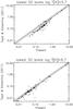 |
Fig. 2 Thermally-averaged collision strengths (Tayal & Zatsarinny 2011 vs. the present ones) for transitions from the ground configuration to the lowest 50 levels only. Dashed lines indicate ±20%. |
Tayal & Zatsarinny (2011) only provided a limited set of transition probabilities, insufficient to build a proper ion model. Additional A-values, as we calculated in Del Zanna (2009b), were added to produce a more complete ion model. The corresponding line intensities are shown in Col. 5.
List of the strongest Fe viii lines.
Table 5 shows significant differences for a few lines. In a number of cases, the differences are mainly due to the different target, as we have discussed above. However, in many cases this is not the case, and the present intensities are increased. We looked at the populations of all the individual levels and found that in these cases the differences are mainly due to the increased excitation rates from the ground configuration, as we saw previously from the global comparison in Fig. 2, and as shown for a sample of transitions in Fig. 3.
The collision strengths of the forbidden transition within the ground configuration are larger than those of the previous calculations. The collision strengths from the ground configuration to most of the 3s2 3p5 3d2 levels are also increased. Three examples are shown in Fig. 3. Of particular relevance are the increased collision strengths for transitions to the 4DJ levels (see e.g. second plot from the top, transition 2−5), which are of particular importance for temperature diagnostic applications.
Finally, we looked at the populations of the highly mixed 3s2 3p5 3d22P3/2 and 3s2 3p6 4p 2P3/2 levels (nos 41 and 43). We found that the populations are partly (30–40%) due to cascading from the 3s2 3p6 4d 2D5/2 level. The population of this 4d level (no. 52) is slightly increased in the present model, because of increased excitation from the ground configuration.
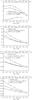 |
Fig. 3 Thermally-averaged collision strengths for a selection of transitions (see text). |
As reviewed in Del Zanna (2009b), there are many observations of Fe viii lines, but only few with sufficient spectral resolution and calibrated line intensities. For example, Malinovsky & Heroux (1973) published a well-calibrated EUV medium-resolution (0.25 Å) integrated-Sun spectrum, but several of the Fe viii lines were significantly blended.
A similar medium-resolution spectrum was obtained in the laboratory with a theta-pinch device by Datla et al. (1975). This spectrum was not as much affected by blends because it was mainly produced by iron. The authors provided two sets of calibrated line intensities. For case a, relative to high temperatures, large disagreements with the present atomic data are found. For case b, where corrections due to optical depth effects were applied, we find excellent greement (within a relative 10%) between predicted and observed line intensities, as shown in Fig. 4. This figure shows the “emissivity ratio” curves 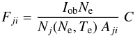 (1)for each line as a function of the electron temperature Te. Iob is the observed intensity of the line (photon units), Nj(Ne,Te) is the population of the upper level j relative to the total number density of the ion, calculated at a fixed density Ne. Aji is the spontaneous radiative transition probability, and C is a scaling constant chosen so the emissivity ratio is near unity. If agreement between experimental and theoretical intensities is present, all lines should be closely spaced. If the plasma is nearly isothermal, all curves should cross at the isothermal temperature.
The emissivities in Fig. 4 were calculated at 1016 cm-3, the measured density at the time of peak intensity of the discharge. The temperature of the plasma was also measured (in an independent way) by Datla et al. (1975) to be about log T [ K ] = 5.7, i.e. in excellent agreement with the crossing of the lines in Fig. 4.
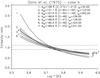 |
Fig. 4 Emissivity ratio curves relative to the Datla et al. (1975) calibrated theta-pinch spectrum (case b). The observed intensities Iob are in ergs. |
A laboratory spectrum with a much higher spectral resolution was obtained by Hasama et al. (1981). It is not clear at which densities the spectrum was taken, however relatively good agreement between predicted and observed intensities is obtained with an electron density of 1018 cm-3, as Fig. 5 shows. The spectrum resolved the decays from the 3s2 3p6 5f 2F7/2,5/2 at 107.869, 108.073 Å, and the decays from the 3s2 3p6 4f 2F7/2,5/2. Excellent agreement (within a few percent) is found in the relative strengths of these decays.
Hasama et al. (1981) noticed in particular that the 167.66 Å line is blended with the two transitions at 168.0 Å. Despite adding the blends, the observed intensity of this line is still much higher than predicted. We note that there are two unidentified transitions from the 3s2 3p4 3d3 configuration (3s2 3p5 3d22H11/2 − 3s2 3p4 3d32H11/2 and 3s2 3p5 3d22H11/2−3s2 3p4 3d32G9/2) which we predict to be relatively strong at 1018 cm-3. If one of these lines was blending the 167.66 Å line, the disagreement would be significantly reduced.
High-resolution EUV solar spectra have been obtained with the Hinode EIS instrument. The identifications and the spectra have been described in Del Zanna (2009a,b). A careful “foreground-subtracted” sunspot loop spectrum was obtained, where Fe viii lines were strong and not blended with hotter lines.
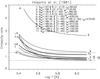 |
Fig. 5 Emissivity ratio curves relative to the Hasama et al. (1981) calibrated spectrum at an electron density of 1018 cm-3. |
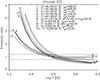 |
Fig. 6 Emissivity ratio curves relative to the “foreground-subtracted” Sunspot loop leg observed by Hinode EIS (Del Zanna 2009a,b). The intensities Iob are in phot cm-2 s-1 arcsec-2. |
Figure 6 shows the curves for the strongest transitions observed by Hinode EIS. We adopted our recent revision of the EIS radiometric calibration (Del Zanna 2013). There is an excellent agreement, to within a relative 10–20% (comparable to the uncertainty in the calibration), between observed and calculated intensities.
Our benchmark work on Fe vii (Del Zanna 2009a) suggested that about 30% of the intensity of the 197.36 Å line would be due to a transition from this ion. We have therefore taken 70% of the observed intensity to produce the emissivity ratio curve for the Fe viii transition, and find excellent agreement with the other curves. This confirms the accuracy of our predicted intensity, that is largely different from what is predicted using Tayal & Zatsarinny (2011) data.
We recall that large discrepancies were found with the Griffin et al. (2000) atomic data (even adjusted), in particular with the strong lines of the 3p6 3d 2DJ − 3p5 3d24DJ transition array. These lines (numbered 7−10 in the figure) are particularly important because they provide, in combination with lines from higher-excitation levels, a direct way to measure the electron temperature. With the previous Griffin et al. (2000) adjusted atomic data, these transitions indicated a much too low temperature of log T [ K ] = 5.4 (Del Zanna 2009b), while now they indicate a temperature of between log T [ K ] = 5.6 and 5.7, i.e. close to that one obtained from an emission measure analysis of the magnesium lines, log T [ K ] = 5.65 by Del Zanna (2009b).
5. Conclusions
We have recently seen in many cases that carrying out a large-scale scattering calculation produces two important effects. The first effect is direct: the collision strengths of some transitions can be increased due to extra resonances. The second effect is more subtle. As we have discovered for other coronal iron ions (Fe x: Del Zanna et al. 2012b; Fe xi: Del Zanna & Storey 2013; Fe xii: Del Zanna et al. 2012a), small increases (due to extra resonances) in the collision strengths of a large number of higher levels can significantly affect, by cascading, the populations of lower levels by as much as 30–40%.
However, carrying out a large-scale scattering calculation does not necessarily produce an accurate result, in particular for highly-mixed levels which give rise to transitions whose oscillator strengths vary significantly, depending on the target description. The most complex case we studied, Fe xi, is a typical example. It took some time to be resolved, because of three highly mixed n = 3, J = 1 levels, which produce some among the strongest EUV lines for this ion. After several attempts, we (Del Zanna et al. 2010) found an ad-hoc target which produced accurate collision strengths for these three n = 3, J = 1 levels. The accuracy was confirmed a posteriori with detailed comparisons against observations (Del Zanna 2010). Later, we performed a larger scattering calculation (Del Zanna & Storey 2013), which significantly improved the atomic data for many lower (within the n = 3) and higher (n = 4) levels, but did not produce accurate collision strengths for these three n = 3, J = 1 levels.
The atomic structure of Fe viii turned out to be far more complex than Fe xi, with several levels being strongly spin-orbit mixed and sensitive to their term separation. It is ultimately very difficult to assess a priori how good a target is, but fortunately our identifications of several new levels (Del Zanna 2009b) for this ion helped the comparison between experimental and theoretical energies.
In this work, we have focused on the main low-lying levels for this ion. We have presented a target that, with the use of the TECs, is an improvement over the targets employed previously. The use of TECs, in fact, provides very satisfactory results, as it has done in the past. We note that, previously, our use of TECs has been confined to describing atomic structure only. Now, we have described how they can be used consistently within the ICFT R-matrix method and have carried-out such a calculation utilizing them. As a consequence, we are planning to revisit and improve upon some previous calculations using this approach.
Finally, we used a selection of laboratory and solar spectra to confirm the reliability of the present atomic data. We find an excellent agreement with the XUV lines observed with a theta-pinch by Datla et al. (1975). The predicted intensities of the strongest Fe viii EUV lines observed by Hinode EIS are now finally in good agreement with observations. The temperature diagnostics pointed out in Del Zanna (2009b) are providing, with the present atomic data, values in close agreement with those obtained from other ions and methods. These Hinode EIS spectral liens therefore now provide a reliable way to measure electron temperatures for the solar corona.
Acknowledgments
The present work was funded by STFC (UK) through the University of Cambridge DAMTP astrophysics grant, and the University of Strathclyde UK APAP network grant ST/J000892/1.
References
- Badnell, N. R. 2011, Comput. Phys. Commun., 182, 1528 [NASA ADS] [CrossRef] [Google Scholar]
- Badnell, N. R., & Griffin, D. C. 2001, J. Phys. B At. Mol. Phys., 34, 681 [NASA ADS] [CrossRef] [Google Scholar]
- Berrington, K. A., Eissner, W. B., & Norrington, P. H. 1995, Comput. Phys. Commun., 92, 290 [NASA ADS] [CrossRef] [Google Scholar]
- Burgess, A. 1974, J. Phys. B At. Mol. Phys., 7, L364 [NASA ADS] [CrossRef] [Google Scholar]
- Burgess, A., & Tully, J. A. 1992, A&A, 254, 436 [NASA ADS] [Google Scholar]
- Burgess, A., Chidichimo, M. C., & Tully, J. A. 1997, J. Phys. B At. Mol. Phys., 30, 33 [NASA ADS] [CrossRef] [Google Scholar]
- Chidichimo, M. C., Badnell, N. R., & Tully, J. A. 2003, A&A, 401, 1177 [NASA ADS] [CrossRef] [EDP Sciences] [Google Scholar]
- Culhane, J. L., Harra, L. K., James, A. M., et al. 2007, Sol. Phys., 60 [Google Scholar]
- Datla, R. U., Blaha, M., & Kunze, H.-J. 1975, Phys. Rev. A, 12, 1076 [NASA ADS] [CrossRef] [Google Scholar]
- Del Zanna, G. 2009a, A&A, 508, 501 [NASA ADS] [CrossRef] [EDP Sciences] [Google Scholar]
- Del Zanna, G. 2009b, A&A, 508, 513 [NASA ADS] [CrossRef] [EDP Sciences] [Google Scholar]
- Del Zanna, G. 2010, A&A, 514, A41 [NASA ADS] [CrossRef] [EDP Sciences] [Google Scholar]
- Del Zanna, G. 2013, A&A, 555, A47 [NASA ADS] [CrossRef] [EDP Sciences] [Google Scholar]
- Del Zanna, G., & Storey, P. J. 2013, A&A, 549, A42 [NASA ADS] [CrossRef] [EDP Sciences] [Google Scholar]
- Del Zanna, G., Berrington, K. A., & Mason, H. E. 2004, A&A, 422, 731 [NASA ADS] [CrossRef] [EDP Sciences] [Google Scholar]
- Del Zanna, G., Storey, P. J., & Mason, H. E. 2010, A&A, 514, A40 [NASA ADS] [CrossRef] [EDP Sciences] [Google Scholar]
- Del Zanna, G., Storey, P. J., Badnell, N. R., & Mason, H. E. 2012a, A&A, 543, A139 [NASA ADS] [CrossRef] [EDP Sciences] [Google Scholar]
- Del Zanna, G., Storey, P. J., Badnell, N. R., & Mason, H. E. 2012b, A&A, 541, A90 [NASA ADS] [CrossRef] [EDP Sciences] [Google Scholar]
- Eissner, W., Jones, M., & Nussbaumer, H. 1974, Comput. Phys. Commun., 8, 270 [NASA ADS] [CrossRef] [Google Scholar]
- Griffin, D. C., Badnell, N. R., & Pindzola, M. S. 1998, J. Phys. B At. Mol. Phys., 31, 3713 [NASA ADS] [CrossRef] [Google Scholar]
- Griffin, D. C., Pindzola, M. S., & Badnell, N. R. 2000, A&AS, 142, 317 [NASA ADS] [CrossRef] [EDP Sciences] [Google Scholar]
- Hasama, T., Onishi, Y., Uchiike, M., & Fukuda, K. 1981, Jpn. J. Appl. Phys., 20, 2269 [NASA ADS] [CrossRef] [Google Scholar]
- Hummer, D. G., Berrington, K. A., Eissner, W., et al. 1993, A&A, 279, 298 [NASA ADS] [Google Scholar]
- Malinovsky, L., & Heroux, M. 1973, ApJ, 181, 1009 [NASA ADS] [CrossRef] [Google Scholar]
- Nussbaumer, H., & Storey, P. J. 1978, A&A, 64, 139 [NASA ADS] [Google Scholar]
- O’Dwyer, B., Del Zanna, G., Badnell, N. R., Mason, H. E., & Storey, P. J. 2012, A&A, 537, A22 [NASA ADS] [CrossRef] [EDP Sciences] [Google Scholar]
- Saraph, H. E. 1972, Comput. Phys. Commun., 3, 256 [Google Scholar]
- Tayal, S. S., & Zatsarinny, O. 2011, ApJ, 743, 206 [NASA ADS] [CrossRef] [Google Scholar]
- Young, P. R., & Landi, E. 2009, ApJ, 707, 173 [NASA ADS] [CrossRef] [Google Scholar]
- Young, P. R., Del Zanna, G., Mason, H. E., et al. 2007, PASJ, 59, 727 [Google Scholar]
- Zeippen, C. J., Seaton, M. J., & Morton, D. C. 1977, MNRAS, 181, 527 [NASA ADS] [CrossRef] [Google Scholar]
- Zeng, J., Jin, F., Zhao, G., & Yuan, J. 2003, J. Phys. B At. Mol. Phys., 36, 3457 [Google Scholar]
All Tables
All Figures
|
Fig. 1 Term energies of the target levels (25 configurations). The lowest 209 terms which produce levels having energies below the dashed line have been retained for the close-coupling expansion. |
| In the text | |
|
Fig. 2 Thermally-averaged collision strengths (Tayal & Zatsarinny 2011 vs. the present ones) for transitions from the ground configuration to the lowest 50 levels only. Dashed lines indicate ±20%. |
| In the text | |
|
Fig. 3 Thermally-averaged collision strengths for a selection of transitions (see text). |
| In the text | |
|
Fig. 4 Emissivity ratio curves relative to the Datla et al. (1975) calibrated theta-pinch spectrum (case b). The observed intensities Iob are in ergs. |
| In the text | |
|
Fig. 5 Emissivity ratio curves relative to the Hasama et al. (1981) calibrated spectrum at an electron density of 1018 cm-3. |
| In the text | |
|
Fig. 6 Emissivity ratio curves relative to the “foreground-subtracted” Sunspot loop leg observed by Hinode EIS (Del Zanna 2009a,b). The intensities Iob are in phot cm-2 s-1 arcsec-2. |
| In the text | |
Current usage metrics show cumulative count of Article Views (full-text article views including HTML views, PDF and ePub downloads, according to the available data) and Abstracts Views on Vision4Press platform.
Data correspond to usage on the plateform after 2015. The current usage metrics is available 48-96 hours after online publication and is updated daily on week days.
Initial download of the metrics may take a while.