| Issue |
A&A
Volume 569, September 2014
|
|
|---|---|---|
| Article Number | L8 | |
| Number of page(s) | 4 | |
| Section | Letters | |
| DOI | https://doi.org/10.1051/0004-6361/201424748 | |
| Published online | 02 October 2014 | |
First spectrally-resolved H2 observations towards HH 54 ⋆
Low H2O abundance in shocks
1
Osservatorio Astrofisico di Arcetri, Largo Enrico Fermi 5,
50125
Florence,
Italy
e-mail:
This email address is being protected from spambots. You need JavaScript enabled to view it.
2
Osservatorio Astronomico di Roma, via di Frascati 33,
00040
Monteporzio Catone,
Italy
3
Niels Bohr Institute, University of Copenhagen,
Juliane Maries Vej
30, 2100
Copenhagen Ø.,
Denmark
4
Centre for Star and Planet Formation and Natural History Museum of
Denmark, University of Copenhagen, Øster Voldgade 5–7, 1350
Copenhagen K.,
Denmark
5
Department of Earth and Space Sciences, Chalmers University of
Technology, Onsala Space Observatory, 439 92
Onsala,
Sweden
6
European Southern Observatory, Karl Schwarzschild str.2, 85748
Garching bei Muenchen,
Germany
7
LERMA, Observatoire de Paris, UMR 8112 of the CNRS, 61 Av. de
l’Observatoire, 75014
Paris,
France
8
ASDC, 00044 Frascati, Roma, Italy
9
The Johns Hopkins University, Baltimore, MD
21218,
USA
10
Observatorio Astronómico Nacional (IGN),
Alfonso XII 3,
28014
Madrid,
Spain
11
Leiden Observatory, Leiden University,
PO Box 9513,
2300 RA
Leiden, The
Netherlands
12
Max Planck Institut für Extraterrestrische Physik (MPE),
Giessenbachstr.1,
85748
Garching,
Germany
Received:
4
August
2014
Accepted:
7
September
2014
Abstract
Context. Herschel observations suggest that the H2O distribution in outflows from low-mass stars resembles the H2 emission. It is still unclear which of the different excitation components that characterise the mid- and near-IR H2 distribution is associated with H2O.
Aims. The aim is to spectrally resolve the different excitation components observed in the H2 emission. This will allow us to identify the H2 counterpart associated with H2O and finally derive directly an H2O abundance estimate with respect to H2.
Methods. We present new high spectral resolution observations of H2 0−0 S(4), 0−0 S(9), and 1−0 S(1) towards HH 54, a bright nearby shock region in the southern sky. In addition, new Herschel/HIFI H2O (212 − 101) observations at 1670 GHz are presented.
Results. Our observations show for the first time a clear separation in velocity of the different H2 lines: the 0−0 S(4) line at the lowest excitation peaks at −7 km s-1, while the more excited 0−0 S(9) and 1−0 S(1) lines peak at −15 km s-1. H2O and high-J CO appear to be associated with the H2 0−0 S(4) emission, which traces a gas component with a temperature of 700−1000 K. The H2O abundance with respect to H2 0−0 S(4) is estimated to be X(H2O) < 1.4 × 10⁻⁵ in the shocked gas over an area of 13′′.
Conclusions. We resolve two distinct gas components associated with the HH 54 shock region at different velocities and excitations. This allows us to constrain the temperature of the H2O emitting gas (≤1000 K) and to derive correct estimates of H2O abundance in the shocked gas, which is lower than what is expected from shock model predictions.
Key words: stars: formation / infrared: ISM / ISM: jets and outflows / Herbig-Haro objects / ISM: individual objects: HH 54
Based on observations made with ESO telescopes at the La Silla Paranal Observatory under programme IDs: 089.C-0772, 292.C-5025.
© ESO, 2014
1. Introduction
Protostellar jets and outflows are a direct consequence of the accretion mechanism in young stellar objects during their earliest phase (e.g. Ray et al. 2007). The interaction between the ejecta and the circumstellar medium occurs via radiative shocks (e.g. Kaufman & Neufeld 1996; Flower & Pineau des Forêts 2010), whose energy is radiated away through emission lines of atomic, ionic, and molecular species. Hot gas at temperatures above 2000 K cools principally through H2 ro-vibrational lines in the near-IR and abundant atomic and ionic species (e.g. Eislöffel et al. 2000; Giannini et al. 2004). Warm gas components at hundreds of Kelvin cool via mid- and far-IR molecular lines, particularly rotational transitions of H2 (at λ ≤ 28 μm) and lines of other molecular species, such as CO and H2O.
H2 transitions observed.
Water has a key role in protostellar environments (van Dishoeck et al. 2011). Its abundance with respect to H2 is expected to increase from <10-7 in cold regions up to 3 × 10⁻⁴ in warm gas due to the combined effects of sputtering of grain mantles and high-temperature reactions (Hollenbach & McKee 1989; Kaufman & Neufeld 1996; Flower & Pineau des Forêts 2010; Suutarinen et al. 2014). The Herschel Space Observatory revealed the complexity of H2O line profiles (e.g. Codella et al. 2010; Kristensen et al. 2012; Santangelo et al. 2012; Vasta et al. 2012) and showed that H2O emission probes warm (≳300 K) and dense (nH2> 105 cm-3) gas with spatial distribution that resembles the H2 emission (e.g. Nisini et al. 2010; Tafalla et al. 2013; Santangelo et al. 2013). Low H2O abundances are derived in outflows for warm shocked gas, ranging from a few ×10-6 to a few ×10-5 (e.g. Bjerkeli et al. 2012; Santangelo et al. 2013; Tafalla et al. 2013; Busquet et al. 2014). These abundance values are at least an order of magnitude lower than what is expected in warm shocked gas from shock model predictions (e.g. Kaufman & Neufeld 1996; Flower & Pineau des Forêts 2010). Their determinations rely on the assumption that H2O traces the same gas as the spectrally unresolved low-J H2 0–0 lines. Spectrally resolved observations of H2 are thus needed to directly compare the line profiles and finally test this hypothesis.
The Herbig-Haro object HH 54 is located in the nearby star-forming region Chamaeleon II (D = 180 pc, Whittet et al. 1997). The object shows a clumpy appearance, consisting of several arcsecond-scale bright knots. Knee (1992) associates HH 54 with a monopolar blue-shifted CO outflow, whose driving source remains unclear (e.g. Caratti o Garatti et al. 2006; Ybarra & Lada 2009; Bjerkeli et al. 2011). Mid-IR cooling is dominated by pure rotational H2 lines (Cabrit et al. 1999; Giannini et al. 2006; Neufeld et al. 1998, 2006) probing warm gas with a mixture of temperatures in the range 400−1200 K. HH 54 was also observed in several lines of CO and H2O from space and the ground (Liseau et al. 1996; Nisini et al. 1996; Bjerkeli et al. 2009, 2011).
In this letter we present new ESO VLT high-resolution spectroscopic observations of H2 towards HH 54. The observations are complemented with Herschel/HIFI observations of H2O (212 − 101). This unique dataset is used to spectrally resolve the different excitation components observed in H2. We are finally able to identify the H2 counterpart associated with H2O and derive the H2O abundance in the shocked gas directly.
2. Observations
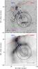 |
Fig. 1 Upper: H2 1−0 S(1) image of HH 54 from NTT/SofI observations (Giannini et al. 2006). The positioning of the slits
adopted for VLT/VISIR and CRIRES observations is shown in blue and red. The beam sizes
of Herschel H2O (212−101) (magenta circle), CO
(15−14) (green, Bjerkeli et al. 2014), and SEST CO (2−1) (black, Bjerkeli et al. 2009, 2011)
are displayed. Offsets are relative to: αJ2000 =
12h55m50 |
Our dataset consists of data collected towards HH 54 with ESO facilities (Table 1) and with Herschel. Figure 1 shows the VLT slit positions and Herschel and SEST beam sizes for the observations presented in this paper in comparison with the H2 1−0 S(1) and 0−0 S(4) maps of the region (Giannini et al. 2006; Neufeld et al. 2006).
2.1. VISIR high-resolution mid-IR spectroscopy
On April 2012 we performed spectrally-resolved observations of H2 0−0 S(4) (see Table 1) with VLT/VISIR (Lagage et al.
2004). The  slit was positioned
on the basis of the Spitzer image (see Fig. 1); it was oriented in a way to encompass knot B, which was covered by the
Herschel single-pointing observations of H2O (see Sect. 2.3), and the C1/C2 knots, which correspond to the
brightest knot in the Spitzer H2 emission. We conducted our observations by chopping and
nodding the telescope off-source, with equal time on both positions. Data reduction and
calibration were performed by using the VISIR pipeline recipes (version 3.5.1)1, which provide standard procedures for flat-fielding
and background subtraction. A model for the sky emission lines is used by the pipeline for
the wavelength calibration. To fit the dispersion relation we employed a second degree
polynomial, which provides higher correlation coefficient with respect to the default
pipeline linear solution. The uncertainty on the peak velocity is about 3
km s-1,
comparable with the spectral pixel. The IRAF package was used for spectra extraction. Only
C1/C2 knots are clearly detected with VISIR; knot M is only tentatively detected in the
spectral image, whereas knot B is not detected.
slit was positioned
on the basis of the Spitzer image (see Fig. 1); it was oriented in a way to encompass knot B, which was covered by the
Herschel single-pointing observations of H2O (see Sect. 2.3), and the C1/C2 knots, which correspond to the
brightest knot in the Spitzer H2 emission. We conducted our observations by chopping and
nodding the telescope off-source, with equal time on both positions. Data reduction and
calibration were performed by using the VISIR pipeline recipes (version 3.5.1)1, which provide standard procedures for flat-fielding
and background subtraction. A model for the sky emission lines is used by the pipeline for
the wavelength calibration. To fit the dispersion relation we employed a second degree
polynomial, which provides higher correlation coefficient with respect to the default
pipeline linear solution. The uncertainty on the peak velocity is about 3
km s-1,
comparable with the spectral pixel. The IRAF package was used for spectra extraction. Only
C1/C2 knots are clearly detected with VISIR; knot M is only tentatively detected in the
spectral image, whereas knot B is not detected.
2.2. CRIRES high-resolution near-IR spectroscopy
We carried out high-dispersion spectroscopic observations of the H2 0−0 S(9) and H2 1−0 S(1) transitions (Table 1) towards HH 54 with VLT/CRIRES (Kaeufl et al. 2004). Observations were performed between January and
February 2014 during director discretionary time. Since only the bright C1/C2 knots were
detected by VISIR, the CRIRES  slit was oriented in
order to cover them (Fig. 1). Chopping and nodding
were performed along the slit to minimise the integration time. Data reduction and
wavelength calibration were performed with the CRIRES pipeline recipes (version 2.3.1).
The wavelength calibration, based on the comparison with a sky emission model, was
satisfactory (high correlation coefficient) for the 0−0 S(9). OH emission lines were used to
refine the wavelength scale for the 1−0 S(1). The uncertainty associated with peak velocities is
~2.5 km s-1. The IRAF package was used for
spectra extraction.
slit was oriented in
order to cover them (Fig. 1). Chopping and nodding
were performed along the slit to minimise the integration time. Data reduction and
wavelength calibration were performed with the CRIRES pipeline recipes (version 2.3.1).
The wavelength calibration, based on the comparison with a sky emission model, was
satisfactory (high correlation coefficient) for the 0−0 S(9). OH emission lines were used to
refine the wavelength scale for the 1−0 S(1). The uncertainty associated with peak velocities is
~2.5 km s-1. The IRAF package was used for
spectra extraction.
2.3. Herschel/HIFI observations
Single-pointing observations of H2O (212−101) at 1669.9 GHz were performed with
the Heterodyne Instrument for the Far Infrared (HIFI, de Graauw et al. 2010) on board Herschel towards HH 54B (see
Fig. 1). The reference coordinates are
αJ2000 =
12h55m50 3,
δJ2000 = −
76°56′23′′. The observations were carried out in September
20122. The diffraction-limited beam size is
~13′′. The data were processed with
the ESA-supported package hipe version 12.0 for calibration. The HebCorrection
and fitHifiFringe tasks within hipe were successfully used to remove the
electronic standing waves in Band 6, which affected the line. Further data reduction and
analysis were performed using the GILDAS3 software.
The antenna temperature scale,
3,
δJ2000 = −
76°56′23′′. The observations were carried out in September
20122. The diffraction-limited beam size is
~13′′. The data were processed with
the ESA-supported package hipe version 12.0 for calibration. The HebCorrection
and fitHifiFringe tasks within hipe were successfully used to remove the
electronic standing waves in Band 6, which affected the line. Further data reduction and
analysis were performed using the GILDAS3 software.
The antenna temperature scale,  , was
converted into the main-beam temperature scale, Tmb, using main-beam efficiency factor
of 0.71 (Roelfsema et al. 2012). The flux
calibration uncertainty is around 10%, based on cross-calibration with
Herschel/PACS (Bjerkeli et al.
2011). At the velocity resolution of 1 km s-1, the rms noise is 80 mK
(Tmb scale).
, was
converted into the main-beam temperature scale, Tmb, using main-beam efficiency factor
of 0.71 (Roelfsema et al. 2012). The flux
calibration uncertainty is around 10%, based on cross-calibration with
Herschel/PACS (Bjerkeli et al.
2011). At the velocity resolution of 1 km s-1, the rms noise is 80 mK
(Tmb scale).
3. Two velocity components in H2 observations
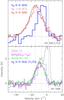 |
Fig. 2 Upper: H2 0−0 S(4) towards HH 54C1/C2 is compared with 1−0 S(1) and 0−0 S(9). Spectra are normalized to their peak values. The vertical dashed line marks the systemic velocity (vLSR = + 2.4 km s-1, Bjerkeli et al. 2011). The two vertical dotted lines indicate the velocity of: the 0−0 S(4) peak at − 7 km s-1; and the 1−0 S(1) and 0−0 S(9) peaks at −15 km s-1. Lower: H2O (212 − 101), CO (15−14), and CO (2−1) towards HH 54B are compared with H2 0−0 S(4) at HH 54C1/C2. H2O, CO, and H2 are normalized to the peak of the bump feature in CO (2−1). |
Velocity centroids of the CRIRES spectra at C1 and C2 knots are consistent within one spectral pixel (<3 km s-1). The two spectra have thus been averaged to compare with VISIR H2 0−0 S(4) extracted at knot C1/C2. The comparison is presented in the upper panel of Fig. 2. A peak velocity of −7 km s-1 is associated with the 0−0 S(4) line, whereas the higher excitation 1−0 S(1) and 0−0 S(9) lines peak at the higher blue-shifted velocity of −15 km s-1. Our spectrally-resolved H2 observations clearly show for the first time that mid-IR and near-IR H2 lines are well separated in velocity, thus representing two distinct velocity components. This suggests that two separate shock components with different excitation conditions are associated with gas peaking at different velocities.
The comparison between H2 0−0 S(4) at HH 54C1/C2 and H2O (212−101), CO (15−14) (Bjerkeli et al. 2014), and CO (2−1) (Bjerkeli et al. 2009, 2011) observations at HH 54B is presented in the lower panel of Fig. 2. The low-J CO lines, in particular CO (2−1), present a two-components profile: a triangular-shaped low-velocity (LV CO, hereafter) component, which peaks at the systemic velocity of the cloud (+2.4 km s-1); and an additional superposed “bump-like” component (Bjerkeli et al. 2011) centred at the blue-shifted velocity of − 7 km s-1. This latter feature seems to dominate the emission of the high-J CO (15−14). The similarity between CO (15−14) and H2O line profiles, taken with similar beam sizes (12′′ and 13′′), suggests that the bump feature is associated with the H2O emitting gas and has higher excitation with respect to the LV gas.
Although the H2 0−0 S(4) spectrum is taken at the C1/C2 knot, the comparison with H2O and high-J CO observed at knot B shows that the three lines trace emission in the same velocity range. Moreover, taking the different spectral resolutions and the uncertainty on the H2 peak velocity determination into account (see Sect. 2.1), the H2 0−0 S(4) line profile well resembles the H2O and high-J CO line profiles (Fig. 2 bottom). HIFI maps of CO (10−9) and lower-J CO lines by Bjerkeli et al. (2011) show that, although the relative intensity of the LV and bump components changes within the HH 54 region, their peak velocities remain constant within 2 km s-1 among the different knots. We thus also assume that the peak velocity of the H2O emission, which appears to be associated with the high-J CO emission at knot B, does not change within the region and in particular along the VISIR slit. In this case, the H2 0−0 S(4) emission would be associated with the same gas as traced by H2O and high-J CO.
In conclusion, our observations detect for the first time the presence of a stratification in velocity in the H2 gas from low- to high-excitation emission lines. The H2 0−0 S(4) component appears to be associated with H2O and high-J CO, as expected from the comparison between the spatial distributions (e.g. Nisini et al. 2010; Tafalla et al. 2013; Santangelo et al. 2013). We note that in the low-J CO an additional gas component around the systemic velocity is detected. This gas component is not observed in the high-J CO lines and in the H2 lines, since higher temperatures are needed to excite them. On the other hand, the higher velocity component associated with H2 1−0 S(1) and 0−0 S(9) is not detected in the CO emission, even in the higher-J lines, since it is associated with a gas at even higher temperatures (T ≳ 2000 K).
4. H2O abundance estimate
Our new observations allow us to spectrally identify the 0−0 S(4) line as the H2 counterpart associated with H2O, with the assumption that the H2 and H2O profiles do not change between the C and B knots. This can be used to accurately constrain the temperature of the gas from the H2 emission and derive correct H2O abundances with respect to H2. Neufeld et al. (2006) mapped H2 S(0)−S(7) pure rotational lines towards HH 54 with Spitzer/IRS. Their H2 rotational diagram, constructed over a 15′′ region encompassing HH 54B, indicates the presence of warm gas with temperatures in the range 400−1200 K. According to these authors, a temperature range of 700−1000 K is associated with the 0−0 S(4) emission, which corresponds N(H2) = 6.6 × 10¹⁹ and 2.1 × 1019 cm-2 over 13′′ for 700 and 1000 K, respectively.
We assumed for the H2O emission the same temperature range as derived from the H2 0−0 S(4) line and a gas density n(H2) ≳ 105 cm-3 (e.g. Tafalla et al. 2013; Santangelo et al. 2013; Busquet et al. 2014). We used the radex molecular LVG radiative transfer code (van der Tak et al. 2007) to model the observed H2O (212 −101) emission. A typical line width of 10 km s-1 was adopted from a Gaussian fitting to the spectrum (see Fig. 2). The lower limit on the H2 density corresponds to an upper limit on the derived column density. In particular, we obtain N(H2O) <3 × 1014 cm-2 over a 13′′ area. The comparison with the H2 column density obtained from the 0−0 S(4) for the same temperature range gives an H2O abundance X(H2O) < 1.4 × 10⁻⁵. A lower H2 density of 2 × 104 cm-3 (Bjerkeli et al. 2011, 2014) would increase the H2O abundance by a factor of 2. The upper level energy of H2O (212−101), which is about 114 K, is much smaller than that of the H2 S(4) line (Table 1). Therefore, we cannot exclude that H2O emission is associated with a colder gas component that is not probed by our H2 observations. However, a temperature lower than the assumed 700−1000 K would indicate an even lower H2O abundance, thus strengthening our result. The derived upper limit on the H2O abundance is in agreement with the abundance value of 10-5 derived by Liseau et al. (1996) and Bjerkeli et al. (2011) from ISO and Herschel observations of transitions at similar wavelengths as well as with the upper limit of < 1.6 × 10⁻⁴ obtained by Neufeld et al. (2006) based on non-detections of shorter wavelength transitions covered by Spitzer. Our H2O abundance estimate in HH 54 confirms the values recently found by Herschel in outflows from Class 0 sources (e.g. Bjerkeli et al. 2012; Santangelo et al. 2013; Tafalla et al. 2013; Busquet et al. 2014), which are based on the assumption that H2O traces the same gas as traced by the low-J H2 emission.
An estimate of the H2O abundance at the C knot can also be derived using the PACS map of H2O (212 − 101) by Bjerkeli et al. (2011). The H2O flux density at knot C is a factor of 2 lower than at the position of the HIFI H2O observations, which yields N(H2O) < 1014 cm-2. The H2 column density obtained from the 0−0 S(4) at knot C is in the range N(H2) = 5 × 10¹⁹−1.6 × 1020 cm-2 for 1000 and 700 K, respectively. The comparison between H2O and H2 indicates an H2O abundance X(H2O) < 2 × 10⁻⁶, which is even more strict than that derived at knot B. This indicates a variation of H2O abundance within the HH 54 region, with a decrease towards the peak of the H2 S(4) emission. This may explain the different emission peaks of the H2O distribution observed by PACS (Bjerkeli et al. 2011) and the H2 S(4) emission.
5. Conclusions
We present new spectrally-resolved observations towards HH 54 of H2 0−0 S(4), 0−0 S(9), and 1−0 S(1). These are complemented by new Herschel/HIFI H2O (212−101) observations. Our data show for the first time the separation in velocity between the gas component traced by the low-excitation H2 0−0 S(4) line and that associated with the H2 lines at higher excitation. The observed H2 stratification in velocity suggests that our observations resolve two distinct gas components associated with the HH 54 shock region at different velocity and excitation. We spectrally identify the H2 0−0 S(4) line as the H2 counterpart of H2O emission. This allows us to constrain the temperature of the H2O emitting gas (≤1000 K). H2O abundance is estimated to be lower than what is expected from shock model predictions by at least one order of magnitude. High spectral resolution observations of different targets are needed to confirm this result.
The data are part of the OT2 program “Herschel observations of the shocked gas in HH 54” (observation ID: 1342251604).
Acknowledgments
We thank VLT astronomers and operators for performing excellent service mode observations at CRIRES and providing excellent support with VISIR. We particularly thank the ESO Director’s Office for the DDT observations with CRIRES. This work was partly supported by ASI–INAF project 01/005/11/0, PRIN INAF 2012 – JEDI, and Italian Ministero dell’Istruzione, Università e Ricerca through the grant Progetti Premiali 2012 – iALMA.
References
- Bjerkeli, P., Liseau, R., Olberg, M., et al. 2009, A&A, 507, 1455 [NASA ADS] [CrossRef] [EDP Sciences] [Google Scholar]
- Bjerkeli, P., Liseau, R., Nisini, B., et al. 2011, A&A, 533, A80 [NASA ADS] [CrossRef] [EDP Sciences] [Google Scholar]
- Bjerkeli, P., Liseau, R., Larsson, B., et al. 2012, A&A, 546, A29 [NASA ADS] [CrossRef] [EDP Sciences] [Google Scholar]
- Bjerkeli, P., Liseau, R., Brinch, C., et al. 2014, A&A, in press, DOI: 10.1051/0004-6361/201424789 [Google Scholar]
- Busquet, G., Lefloch, B., Benedettini, M., et al. 2014, A&A, 561, A120 [NASA ADS] [CrossRef] [EDP Sciences] [Google Scholar]
- Cabrit, S., Bontemps, S., et al. 1999, The Universe as Seen by ISO, 427, 449 [NASA ADS] [Google Scholar]
- Caratti o Garatti, A., Giannini, T., Nisini, B., et al. 2006, A&A, 449, 1077 [NASA ADS] [CrossRef] [EDP Sciences] [Google Scholar]
- Codella, C., Lefloch, B., Ceccarelli, C., et al. 2010, A&A, 518, L112 [NASA ADS] [CrossRef] [EDP Sciences] [Google Scholar]
- de Graauw, T., Helmich, F. P., Phillips, T. G., et al. 2010, A&A, 518, L6 [NASA ADS] [CrossRef] [EDP Sciences] [Google Scholar]
- Eislöffel, J., Smith, M. D., & Davis, C. J. 2000, A&A, 359, 1147 [NASA ADS] [Google Scholar]
- Flower, D. R., & Pineau des Forêts, G. 2010, MNRAS, 406, 1745 [NASA ADS] [Google Scholar]
- Giannini, T., McCoey, C., Caratti o Garatti, A., et al. 2004, A&A, 419, 999 [NASA ADS] [CrossRef] [EDP Sciences] [Google Scholar]
- Giannini, T., McCoey, C., Nisini, B., et al. 2006, A&A, 459, 821 [NASA ADS] [CrossRef] [EDP Sciences] [Google Scholar]
- Hollenbach, D., & McKee, C. F. 1989, ApJ, 342, 306 [NASA ADS] [CrossRef] [Google Scholar]
- Kaeufl, H.-U., Ballester, P., Biereichel, P., et al. 2004, Proc. SPIE, 5492, 1218 [CrossRef] [Google Scholar]
- Kaufman, M. J., & Neufeld, D. A. 1996, ApJ, 456, 611 [NASA ADS] [CrossRef] [Google Scholar]
- Knee, L. B. G. 1992, A&A, 259, 283 [NASA ADS] [Google Scholar]
- Kristensen, L. E., van Dishoeck, E. F., Bergin, E. A., et al. 2012, A&A, 542, A8 [NASA ADS] [CrossRef] [EDP Sciences] [Google Scholar]
- Lagage, P. O., Pel, J. W., Authier, M., et al. 2004, The Messenger, 117, 12 [NASA ADS] [Google Scholar]
- Liseau, R., Ceccarelli, C., Larsson, B., et al. 1996, A&A, 315, L181 [NASA ADS] [Google Scholar]
- Neufeld, D. A., Melnick, G. J., & Harwit, M. 1998, ApJ, 506, L75 [NASA ADS] [CrossRef] [Google Scholar]
- Neufeld, D. A., Melnick, G. J., Sonnentrucker, P., et al. 2006, ApJ, 649, 816 [NASA ADS] [CrossRef] [Google Scholar]
- Nisini, B., Lorenzetti, D., Cohen, M., et al. 1996, A&A, 315, L321 [NASA ADS] [Google Scholar]
- Nisini, B., Benedettini, M., Codella, C., et al. 2010, A&A, 518, L120 [NASA ADS] [CrossRef] [EDP Sciences] [Google Scholar]
- Nisini, B., Santangelo, G., Antoniucci, S., et al. 2013, A&A, 549, A16 [NASA ADS] [CrossRef] [EDP Sciences] [Google Scholar]
- Ray, T., Dougados, C., Bacciotti, F., et al. 2007, Protostars and Planets V, 231 [Google Scholar]
- Roelfsema, P. R., Helmich, F. P., Teyssier, D., et al. 2012, A&A, 537, A17 [NASA ADS] [CrossRef] [EDP Sciences] [Google Scholar]
- Santangelo, G., Nisini, B., Giannini, T., et al. 2012, A&A, 538, A45 [NASA ADS] [CrossRef] [EDP Sciences] [Google Scholar]
- Santangelo, G., Nisini, B., Antoniucci, S., et al. 2013, A&A, 557, A22 [NASA ADS] [CrossRef] [EDP Sciences] [Google Scholar]
- Suutarinen, A. N., Kristensen, L. E., et al. 2014, MNRAS, 440, 1844 [NASA ADS] [CrossRef] [Google Scholar]
- Tafalla, M., Liseau, R., Nisini, B., et al. 2013, A&A, 551, A116 [NASA ADS] [CrossRef] [EDP Sciences] [Google Scholar]
- van der Tak, F. F. S., Black, J. H., Schöier, F. L., et al. 2007, A&A, 468, 627 [NASA ADS] [CrossRef] [EDP Sciences] [Google Scholar]
- van Dishoeck, E. F., Kristensen, L. E., Benz, A. O., et al. 2011, PASP, 123, 138 [NASA ADS] [CrossRef] [Google Scholar]
- Vasta, M., Codella, C., Lorenzani, A., et al. 2012, A&A, 537, A98 [NASA ADS] [CrossRef] [EDP Sciences] [Google Scholar]
- Whittet, D. C. B., Prusti, T., Franco, G. A. P., et al. 1997, A&A, 327, 1194 [NASA ADS] [Google Scholar]
- Ybarra, J. E., & Lada, E. A. 2009, ApJ, 695, L120 [NASA ADS] [CrossRef] [Google Scholar]
All Tables
All Figures
|
Fig. 1 Upper: H2 1−0 S(1) image of HH 54 from NTT/SofI observations (Giannini et al. 2006). The positioning of the slits
adopted for VLT/VISIR and CRIRES observations is shown in blue and red. The beam sizes
of Herschel H2O (212−101) (magenta circle), CO
(15−14) (green, Bjerkeli et al. 2014), and SEST CO (2−1) (black, Bjerkeli et al. 2009, 2011)
are displayed. Offsets are relative to: αJ2000 =
12h55m50 |
| In the text | |
|
Fig. 2 Upper: H2 0−0 S(4) towards HH 54C1/C2 is compared with 1−0 S(1) and 0−0 S(9). Spectra are normalized to their peak values. The vertical dashed line marks the systemic velocity (vLSR = + 2.4 km s-1, Bjerkeli et al. 2011). The two vertical dotted lines indicate the velocity of: the 0−0 S(4) peak at − 7 km s-1; and the 1−0 S(1) and 0−0 S(9) peaks at −15 km s-1. Lower: H2O (212 − 101), CO (15−14), and CO (2−1) towards HH 54B are compared with H2 0−0 S(4) at HH 54C1/C2. H2O, CO, and H2 are normalized to the peak of the bump feature in CO (2−1). |
| In the text | |
Current usage metrics show cumulative count of Article Views (full-text article views including HTML views, PDF and ePub downloads, according to the available data) and Abstracts Views on Vision4Press platform.
Data correspond to usage on the plateform after 2015. The current usage metrics is available 48-96 hours after online publication and is updated daily on week days.
Initial download of the metrics may take a while.