| Issue |
A&A
Volume 567, July 2014
|
|
|---|---|---|
| Article Number | A46 | |
| Number of page(s) | 7 | |
| Section | Galactic structure, stellar clusters and populations | |
| DOI | https://doi.org/10.1051/0004-6361/201423813 | |
| Published online | 08 July 2014 | |
Conditions of consistency for multicomponent stellar systems
II. Is a point-axial symmetric model suitable for the Galaxy?
Dept. Matemàtica Aplicada IV, Universitat Politècnica de
Catalunya,
08034 Barcelona,
Catalonia,
Spain
e-mail:
This email address is being protected from spambots. You need JavaScript enabled to view it.
Received:
14
March
2014
Accepted:
14
April
2014
Abstract
Under a common potential, a finite mixture of ellipsoidal velocity distributions satisfying the Boltzmann collisionless equation provides a set of integrability conditions that may constrain the population kinematics. They are referred to as conditions of consistency and were discussed in a previous paper on mixtures of axisymmetric populations. As a corollary, these conditions are now extended to point-axial symmetry, that is, point symmetry around the rotation axis or bisymmetry, by determining which potentials are connected with a more flexible superposition of stellar populations. Under point-axial symmetry, the potential is still axisymmetric, but the velocity and mass distributions are not necessarily. A point-axial stellar system is, in a natural way, consistent with a flat velocity distribution of a disc population. Therefore, no additional integrability conditions are required to solve the Boltzmann collisionless equation for such a population. For other populations, if the potential is additively separable in cylindrical coordinates, the populations are not kinematically constrained, although under point-axial symmetry, the potential is reduced to the harmonic function, which, for the Galaxy, is proven to be non-realistic. In contrast, a non-separable potential provides additional conditions of consistency. When mean velocities for the populations are unconstrained, the potential becomes quasi-stationary, being a particular case of the axisymmetric model. Then, the radial and vertical mean velocities of the populations can differ and produce an apparent vertex deviation of the whole velocity distribution. However, single population velocity ellipsoids still have no vertex deviation in the Galactic plane and no tilt in their intersection with a meridional Galactic plane. If the thick disc and halo ellipsoids actually have non-vanishing tilt, as the surveys of the solar neighbourhood that include RAdial Velocity Experiment (RAVE) data seem to show, the point-axial model is unable to fit the local velocity distribution. Conversely, the axisymmetric model is capable of making a better approach. If, in the end, more accurate data confirm a negligible tilt of the populations, then the point-axisymmetric model will be able to describe non-axisymmetric mass and velocity distributions, although in the Galactic plane the velocity distribution will still be axisymmetric.
Key words: galaxies: kinematics and dynamics / solar neighborhood / galaxies: statistics
© ESO, 2014
1. Introduction
The purpose of the present work is to complete some aspects of the analysis of conditions of consistency for mixtures of axisymmetric stellar systems (Cubarsi 2014, hereafter Paper I) by studying the more general point-axial symmetry (or bisymmetry) case, i.e., rotational symmetry of 180° for the potential and the phase space density functions.
To simplify the solution of the Boltzmann collisionless equation (BCE) it is necessary to introduce some symmetries for the mass and the velocity distributions, such as the assumptions of axisymmetry, steady state, or Galactic plane of symmetry. These hypotheses provide serious limitations for describing in a realistic way the kinematic observables of the Galaxy unless a mixture model is assumed. The conditions of consistency are integrability conditions allowing for a mixture of independent populations of generalised Schwarzschild type to share the same potential function. Since the potential may depend on the population parameters involved in the velocity distribution, the less the potential depends on them, the less kinematically constrained the populations will be.
Several kinematic analyses using the newest radial velocity data from the RAdial Velocity Experiment (RAVE) survey (Siebert et al. 2011; Zwitter et al. 2008; Steinmetz et al. 2006) confirmed that the thin disc has non-vanishing vertex deviation, the thick disc has a radial mean motion differing from that of the thin disc, and the halo velocity ellipsoid is likely to be tilted (e.g., Pasetto et al. 2012a,b; Moni Bidin et al. 2012; Casetti-Dinescu et al. 2011; Carollo et al. 2010; Smith et al. 2009a,b).
It was suggested (Pasetto et al. 2012b; Steinmetz 2012) that the axisymmetry assumption should be relaxed towards a model with point-axial symmetry to account for these features. However, in Paper I we proved that an axisymmetric mixture model is able to describe the actual velocity distribution in the solar neighbourhood provided that the potential is quasi-stationary1 and the phase space density function is time-dependent. This family of potentials is consistent with populations having different mean velocities producing a non-null vertex deviation of the disc distribution. In addition, if the potential is separable in cylindrical coordinates, the velocity ellipsoids may have an arbitrary tilt.
Unlike in the axisymmetric model, in steady state point-axial systems, non-null radial and vertical differential motions are also possible (Sanz-Subirana 1987; Juan-Zornoza 1995). Point-axial symmetry is indeed not a relaxation of the axial symmetry, but a more informative symmetry which may account for ellipsoidal, spiral, or bar structures, and includes axial symmetry as a degenerate case. In particular, along with a quadratic velocity distribution, a point-axial symmetry model provides triaxial mass distributions and velocity ellipsoids with non-vanishing vertex deviation. However, a quadratic point-axial velocity distribution is still symmetric in the peculiar velocities, so that it has null odd-order central moments. Therefore, either in axial or in point-axial symmetric systems, a mixture model is compulsory to fit the full set of local velocity moments. Nevertheless, if each population of the mixture had a velocity ellipsoid with an arbitrary orientation, as, in principle, in the point-axial model, a lower number of populations would likely be required to fit the overall velocity distribution.
Hereafter, this analysis is organised as follows. In the next two sections we review the solution of the BCE for a single point-axial population. In a first step, Chandrasekhar’s system of equations provides the kinematic parameters involved in the velocity distribution function whilst, in a second step, they provide an axisymmetric potential. In the fourth section we find the general solution for the potential, in both the separable and non-separable cases. In the fifth section we study the conditions of consistency for point-axisymmetric mixtures. In the last section we discuss the results in contrast to the axisymmetric case.
2. Point-axial system
For fixed position and time (r,t), a single stellar population is usually described through a Gaussian velocity distribution function, which is a particular case of a generalised quadratic velocity distribution function in terms of the peculiar velocities (u1,u2,u3), that is, f(Q + σ) with Q = ∑ i,jAij(r,t) uiuj, where Aij are the elements of a symmetric, positive definite second-rank tensor. Under point-axial symmetry these functions satisfy, in cylindrical coordinates, Aij(ϖ,θ,z,t) = Aij(ϖ,θ + π,z,t), likewise the function σ and the components of the mean velocity v.
For the above generalised Schwarzschild velocity distribution, the BCE yields the
Chandrasekhar equations (Chandrasekhar 1960), which
are equivalent to the moment equations (Cubarsi 2007,
2010). Their solution provides the tensor
A, the function
σ, the mean
velocity v, and the potential U. The two first
Chandrasekhar equations are Eqs. (1) and (2) in Paper I, that may be written, with the
notation used in Paper I and using the variable Δ = A·v, as
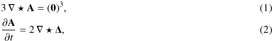 which
yield the elements of the second-rank tensor A and the vector Δ. In the point-axial model these
elements have the functional form (Juan-Zornoza et al. 1990; Juan-Zornoza & Sanz-Subirana 1991)
which
yield the elements of the second-rank tensor A and the vector Δ. In the point-axial model these
elements have the functional form (Juan-Zornoza et al. 1990; Juan-Zornoza & Sanz-Subirana 1991) ![Mathematical equation: \begin{equation} \begin{array}{l}\label{As} A_{\varpi \varpi}=K_1+K_4z^2;\quad A_{\varpi \theta}=\frac12(K'_1+K'_4z^2);\\ [2mm] A_{\varpi z}=-K_4\varpi z;\quad A_{\theta \theta}=K^*_1+k_2\varpi^2+K^*_4z^2; \\[2mm] A_{\theta z}=-\frac12 K'_4 \varpi z; \quad A_{z z}=k_3+K_4\varpi^2; \end{array} \end{equation}](/articles/aa/full_html/2014/07/aa23813-14/aa23813-14-eq16.png) (3)and
(3)and
 (4)with
![Mathematical equation: \begin{equation} \begin{array}{l}\label{Kas} K_1=k_1+q \sin(2\theta+\varphi_1);\quad K^*_1=k_1-q \sin(2\theta+\varphi_1);\\[2mm] K_4=k_4+n \sin(2\theta+\varphi_2);\quad K^*_4=k_4-n \sin(2\theta+\varphi_2); \end{array} \end{equation}](/articles/aa/full_html/2014/07/aa23813-14/aa23813-14-eq18.png) (5)where
k1,k3,q,ϕ1
are time dependent functions and k2,k4,n,
ϕ2,β constants. The
condition that A is
positive-definite implies that k1,k3
are positive functions and k2,k4
non-negative constants, with the requirements k1>q ≥
0, k4>n ≥
0. If K4 is null, the velocity distribution is
independent from z and, in addition, if k2 is null, then
it is independent from ϖ too, which makes no sense in a three-dimensional and
finite Galaxy. Thus, in general, these constants are assumed to be positive, with the
exception of the limiting case K4 = 0 of a two-dimensional disc
distribution2. The particular case k2 = 0 will not be
considered here, although it is discussed at the end of the Conclusions section. It would
correspond to a particular stellar component with constant angular rotation at fixed height
z, similarly
to the axisymmetric model.
(5)where
k1,k3,q,ϕ1
are time dependent functions and k2,k4,n,
ϕ2,β constants. The
condition that A is
positive-definite implies that k1,k3
are positive functions and k2,k4
non-negative constants, with the requirements k1>q ≥
0, k4>n ≥
0. If K4 is null, the velocity distribution is
independent from z and, in addition, if k2 is null, then
it is independent from ϖ too, which makes no sense in a three-dimensional and
finite Galaxy. Thus, in general, these constants are assumed to be positive, with the
exception of the limiting case K4 = 0 of a two-dimensional disc
distribution2. The particular case k2 = 0 will not be
considered here, although it is discussed at the end of the Conclusions section. It would
correspond to a particular stellar component with constant angular rotation at fixed height
z, similarly
to the axisymmetric model.
The uppercase letter K is used for a function also depending on θ. The accents mean derivatives with respect to the angle and the dots with respect to the time. As expected, the functional form of A is similar to the axisymmetric case in Paper I, with the difference that some parameters, those written in capital letters, have an additional term depending on cos2θ and sin2θ, responsible for the rotational symmetry of order 2.
As in the axisymmetric case, the model also provides a time dependent parameter k5 that determines a plane of symmetry for the tensor A at z = − k5/k4. Without loss of generality (Camm 1941) this symmetry plane may be assumed as the Galactic plane, being fixed by taking k5 = 0, resulting then in a symmetric velocity distribution about this plane. Therefore, the point-axisymmetric model, with the inherent symmetry plane, also possesses point-to-point central symmetry.
3. Equations for the potential
The remaining Chandrasekhar equations are Eqs. (3) and (4) in Paper I, which provide the
potential U and
the function σ.
They can be written more easily by using the variable
 as follows:
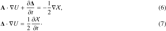 By
elimination of
By
elimination of  between Eqs. (6)and (7), with the new variables
 and
and
 , which are
appropriate to the symmetry plane of the system, six second-order partial differential
equations for the potential are obtained. In their vector notation they can be found in
Chandrasekhar (1960, Eqs. (3.448) and (3.450), p.100).
After substitution of the elements of A and the components of Δ, Sanz-Subirana (1987) and Juan-Zornoza (1995) proved that continuity conditions on the function
force the potential to be axisymmetric. A similar result was obtained by Vandervoort (1979) for point-axial systems, which he called galactic
bars, although the study was limited to a two-dimensional disc with a steady-state
potential.
, which are
appropriate to the symmetry plane of the system, six second-order partial differential
equations for the potential are obtained. In their vector notation they can be found in
Chandrasekhar (1960, Eqs. (3.448) and (3.450), p.100).
After substitution of the elements of A and the components of Δ, Sanz-Subirana (1987) and Juan-Zornoza (1995) proved that continuity conditions on the function
force the potential to be axisymmetric. A similar result was obtained by Vandervoort (1979) for point-axial systems, which he called galactic
bars, although the study was limited to a two-dimensional disc with a steady-state
potential.
3.1. The potential is axisymmetric
These equations are explicitly written in the Appendix. Their solution is tedious and long, and, unfortunately, the above-mentioned thesis papers cannot be accessed easily. Since this is one of the key properties of the point-axial model, we shall see a shorter and alternative justification to this crucial fact.
We note that in the Galactic plane ζ = 0, the three Eqs. (28)–(30)in the Appendix are reduced to Eq. (30)by providing the basic dependence of the potential on the radius and the
angle variables. Hence, we focus on this equation in its complete form. First, we consider
the main case  , hence q ≠ 0, since if
K1 does not depend on θ, the velocity
distribution has no vertex deviation in the Galactic plane3, which was one of the most important observables that justified trying a
non-cylindrical model.
, hence q ≠ 0, since if
K1 does not depend on θ, the velocity
distribution has no vertex deviation in the Galactic plane3, which was one of the most important observables that justified trying a
non-cylindrical model.
If  is non-null,
we write Eq. (30)as
is non-null,
we write Eq. (30)as ![Mathematical equation: \begin{equation} \label{tot33} \begin{array}{l} \frac{\partial^2 U}{\partial \theta^2}- 2\frac{4k_2\tau+(K_1-K_1^*)+2(K_4-K_4^*)\zeta}{K'_1+2K'_4\zeta} \frac{\partial U}{\partial \theta} = 4\tau^2\left[ \frac{\partial^2 U}{\partial \tau^2}- \frac{2 K'_4 \zeta}{K'_1+2K'_4\zeta} \frac{\partial^2 U}{\partial \tau \partial \zeta}\right]\\[2mm] +4\tau\frac{2k_2\tau-(K_1-K_1^*)-2(K_4-K_4^*)\zeta}{K'_1+2K'_4\zeta} \frac{\partial^2 U}{\partial \tau \partial \theta} +\frac{8K_4\tau\zeta}{K'_1+2K'_4\zeta} \frac{\partial^2 U}{\partial\zeta \partial \theta}\cdot \end{array} \end{equation}](/articles/aa/full_html/2014/07/aa23813-14/aa23813-14-eq49.png) (8)We
define the function
(8)We
define the function  and
bear in mind that the continuity and differentiability of the potential, at least up to
the second derivative, implies that V is also differentiable. In the Galactic plane,
the foregoing equation becomes
and
bear in mind that the continuity and differentiability of the potential, at least up to
the second derivative, implies that V is also differentiable. In the Galactic plane,
the foregoing equation becomes 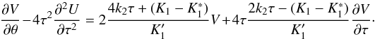 (9)Since
K1 is a π-periodic function of the
angle, a simple recall to the mean value theorem provides us with a value θ0 ∈ [
0,π) for which
(9)Since
K1 is a π-periodic function of the
angle, a simple recall to the mean value theorem provides us with a value θ0 ∈ [
0,π) for which  . Then, if V and
 are non-null functions, in order to avoid any singularity, the right-hand side member of
the above equation must vanish, at least for θ = θ0. We see that the
potential does not satisfy
are non-null functions, in order to avoid any singularity, the right-hand side member of
the above equation must vanish, at least for θ = θ0. We see that the
potential does not satisfy 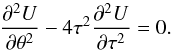 If
so, the solution would be that of the wave equation in the new variable x = lnτ,
hence the solution satisfies U
= F1(x + 2θ) +
F2(x −
2θ), but the potential is a one-valued function and a
periodic function of θ with period42π; therefore, U(x + 2θ)
= U(x + 2(θ + 2kπ))
= U((x + 4kπ) +
2θ) is fulfilled for all k ∈ Z. However, as the
Galaxy is of finite extent, such a potential taking the same value at all points
x +
4kπ is unrealistic.
If
so, the solution would be that of the wave equation in the new variable x = lnτ,
hence the solution satisfies U
= F1(x + 2θ) +
F2(x −
2θ), but the potential is a one-valued function and a
periodic function of θ with period42π; therefore, U(x + 2θ)
= U(x + 2(θ + 2kπ))
= U((x + 4kπ) +
2θ) is fulfilled for all k ∈ Z. However, as the
Galaxy is of finite extent, such a potential taking the same value at all points
x +
4kπ is unrealistic.
On the other hand, the right-hand side of Eq. (9)is non-null. If so, it would be a linear and homogeneous differential equation
in V, with
solution 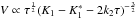 ,
which is discontinuous at
,
which is discontinuous at  .
In particular, when , according to Eq. (5), the singularity takes place at
.
In particular, when , according to Eq. (5), the singularity takes place at
 .
It is worth noticing that for k2 = 0 such a singularity does not
exist, so that we might have non-cylindrical potentials in that degenerate case.
Therefore, the only admissible, continuous, and differentiable solutions to Eq. (9)are axisymmetric potentials satisfying
V = 0,
otherwise, in the Galactic plane, the potential is not differentiable.
.
It is worth noticing that for k2 = 0 such a singularity does not
exist, so that we might have non-cylindrical potentials in that degenerate case.
Therefore, the only admissible, continuous, and differentiable solutions to Eq. (9)are axisymmetric potentials satisfying
V = 0,
otherwise, in the Galactic plane, the potential is not differentiable.
This means that, the axial symmetry is the way that the differential equations for the
potential avoid the singularity produced by any root of the function
. It is
actually a situation similar to the axisymmetric model, where the equations for the
potential, in the quasi-stationary case in Paper I, did avoid the singularity produced by
the zero of the time-dependent function  by providing a solution that does not depend on
  .
.
The case where is null,
consequently  also
vanishes, requires that
also
vanishes, requires that  be non-null,
otherwise the velocity distribution is axisymmetric. Similarly, as in the above case,
there is also an angle θ1 for which
be non-null,
otherwise the velocity distribution is axisymmetric. Similarly, as in the above case,
there is also an angle θ1 for which
 that would produce a
singularity in the solution of Eq. (8), for
ζ ≠ 0,
unless the potential is axisymmetric5.
that would produce a
singularity in the solution of Eq. (8), for
ζ ≠ 0,
unless the potential is axisymmetric5.
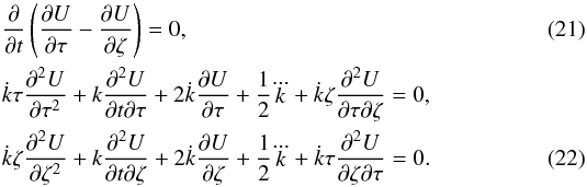
4. Potential
Therefore, in a rotating point-axial system, the potential consistent with a quadratic
velocity distribution is still axisymmetric. The set of partial differential equations for
the potential in the Appendix generalises the ones for the axisymmetric model in Paper I. We
write these equations once they are simplified by taking advantage of the potential
satisfying  . The
first three equations, derived from Eqs. (28)–(30), are
. The
first three equations, derived from Eqs. (28)–(30), are ![Mathematical equation: \begin{equation} \begin{array}{l} 2 K_4\left[2 \left( \frac{\partial U}{\partial \tau}-\frac{\partial U}{\partial \zeta} \right)+ \tau \frac{\partial}{\partial\tau} \left( \frac{\partial U}{\partial \tau}-\frac{\partial U}{\partial \zeta} \right) +\zeta \frac{\partial}{\partial \zeta} \left( \frac{\partial U}{\partial \tau}-\frac{\partial U}{\partial \zeta} \right)\right] \\[2mm] +(K_1-k_3) \frac{\partial^2 U}{\partial \tau \partial \zeta}=0, \end{array} \label{ch01} \end{equation}](/articles/aa/full_html/2014/07/aa23813-14/aa23813-14-eq77.png) (10)
(10)
![Mathematical equation: \begin{equation} \begin{array}{c} 2 K'_4 \left[2 \left( \frac{\partial U}{\partial \tau}-\frac{\partial U}{\partial \zeta} \right)+ \zeta \frac{\partial}{\partial \zeta}\left( \frac{\partial U}{\partial \tau}-\frac{\partial U}{\partial \zeta} \right)\right]+ K'_1 \frac{\partial^2 U}{\partial \tau \partial \zeta}=0, \end{array} \label{ch02} \end{equation}](/articles/aa/full_html/2014/07/aa23813-14/aa23813-14-eq78.png) (11)
(11)
 (12)The
remaining three equations, obtained from Eqs. (31)–(33), are
(12)The
remaining three equations, obtained from Eqs. (31)–(33), are ![Mathematical equation: \begin{equation} \begin{array}{l} 2 K_4 \zeta \frac{\partial}{\partial t}\left( \frac{\partial U}{\partial \tau}-\frac{\partial U}{\partial \zeta} \right) \\[2mm] +\dot{K_1} \tau \frac{\partial^2 U}{\partial \tau^2}+ K_1 \frac{\partial^2 U}{\partial t \partial \tau} + 2 \dot{K_1} \frac{\partial U}{\partial \tau} +\frac12 \dddot{K_1} + \dot{k_3} \zeta \frac{\partial^2 U}{\partial \tau \partial \zeta}=0, \end{array} \label{ch04} \end{equation}](/articles/aa/full_html/2014/07/aa23813-14/aa23813-14-eq80.png) (13)
(13)
![Mathematical equation: \begin{equation} \begin{array}{l} 2 K_4 \tau \frac{\partial}{\partial t}\left( \frac{\partial U}{\partial \zeta}-\frac{\partial U}{\partial \tau} \right) \\[2mm] +\dot{k_3} \zeta \frac{\partial^2 U}{\partial \zeta^2}+ k_3 \frac{\partial^2 U}{\partial t \partial \zeta} + 2 \dot{k_3} \frac{\partial U}{\partial \zeta} +\frac12 \dddot{k_3} + \dot{K_1} \tau \frac{\partial^2 U}{\partial \zeta \partial \tau}=0, \end{array} \label{ch05} \end{equation}](/articles/aa/full_html/2014/07/aa23813-14/aa23813-14-eq81.png) (14)
(14)
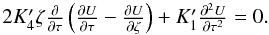
 (15)However,
Eqs. (11)and (12)can be simplified further. By taking the θ-derivative in Eq. (10)and subtracting from Eq. (11), we get
(15)However,
Eqs. (11)and (12)can be simplified further. By taking the θ-derivative in Eq. (10)and subtracting from Eq. (11), we get 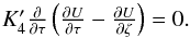 (16)Also, by taking into
account Eq. (12), we get
(16)Also, by taking into
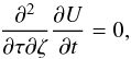
account Eq. (12), we get  (17)Similarly,
Eq. (15)can be expressed in a simpler form.
By taking the θ-derivative in Eq. (13)and subtracting from Eq. (15)we get
(17)Similarly,
Eq. (15)can be expressed in a simpler form.
By taking the θ-derivative in Eq. (13)and subtracting from Eq. (15)we get  , which does not add any new
condition to the previous equation.
, which does not add any new
condition to the previous equation.
Therefore, the equations for the potential in the pont-axial model are the set of Eqs.
(10)–(14), which are similar to the ones of the axial case (Paper I, Eqs.
(7)–(9)), with the additional integrability conditions given by Eqs. (16)and (17). We note that the equations for the potential do not depend on the parameters
 and
and
 . Under axial
symmetry, the conditions depending on the θ-derivatives
. Under axial
symmetry, the conditions depending on the θ-derivatives  and
and
 are identically null. Thus, in a
mixture model these equations are similarly planned for each population component, and
depend on the respective population parameters K1(θ,t), k3(t), and K4(θ).
are identically null. Thus, in a
mixture model these equations are similarly planned for each population component, and
depend on the respective population parameters K1(θ,t), k3(t), and K4(θ).
In the axisymmetric case, when applying the conditions of consistency for a flat velocity distribution, that is, for a potential independent from the population parameter K4, the potential becomes dramatically simplified. In the point-axial case, we shall see that a similar reasoning and solution are inherent to the point-axial symmetry assumption, since the reasoning can be done in regard to the angle dependence as well as to the population dependence of the parameters. In other words, a point-axial system is consistent with a flat velocity distribution unless it degenerates towards an axisymmetric system.
Thus, being at least one of the population parameters K1,K4
functions of the angle θ (otherwise the system is axisymmetric), Eq. (10), once divided by K4, becomes
separated into two parts, one independent from θ and the other depending on θ, which must be null
separately6, 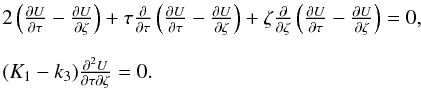 (18)These
equations are equivalent to the conditions of a potential independent from K4 in Paper I,
Eqs. (12) and (14). The latter equation leads to the two typical cases of a potential
additively separable in cylindrical coordinates, or a non-separable potential.
(18)These
equations are equivalent to the conditions of a potential independent from K4 in Paper I,
Eqs. (12) and (14). The latter equation leads to the two typical cases of a potential
additively separable in cylindrical coordinates, or a non-separable potential.
4.1. Separable potential
The separable potential satisfies  In
the point-axial model, at least one of the parameters K1 or
K4 depends on the angle. In particular, if
In
the point-axial model, at least one of the parameters K1 or
K4 depends on the angle. In particular, if
 , owing
to Eq. (11), the potential must be
separable, otherwise
, owing
to Eq. (11), the potential must be
separable, otherwise  would
be held, rendering the axisymmetric model.
would
be held, rendering the axisymmetric model.
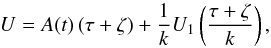
For a separable potential, either with null or
non-null, we are led to the same equations as for the axisymmetric case in Paper I, Eq.
(15), with the addition of Eqs. (16)and
(17), which add the new condition
 , yielding a separable potential
in their harmonic form
, yielding a separable potential
in their harmonic form 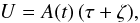 (19)where continuity
conditions in the Galactic plane have been applied in order to neglect the term
proportional to
(19)where continuity
conditions in the Galactic plane have been applied in order to neglect the term
proportional to  .
Therefore, the separable potential reduces to the simple case of the harmonic function,
and does not depend on the population kinematic parameters except for the unique function
A(t) discussed in Paper I.
.
Therefore, the separable potential reduces to the simple case of the harmonic function,
and does not depend on the population kinematic parameters except for the unique function
A(t) discussed in Paper I.
Hence, under a separable potential, the kinematics of a point-axial symmetric system is totally free from conditions of consistency in regard to a mixture of populations. The population’s mean velocities, the semiaxes of the velocity ellipsoids, and their orientations remain unconstrained.
4.2. Non-separable potential
The non-separable potential satisfies  and
and
 Then,
.
According to Eqs. (16)and (17), the point-axial symmetry assumption
requires
Then,
.
According to Eqs. (16)and (17), the point-axial symmetry assumption
requires  . Hence, Eqs. (11)and (12)provide the conditions
 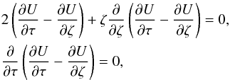 (20)which
separate Eq. (18)into two identically null
equations. Hence, we can consider only one of them. Similarly, the same reasoning of the
preceeding section (either in regard to the dependency on the angle or on the population)
applied to Eqs. (13)–(15)yields the conditions
(20)which
separate Eq. (18)into two identically null
equations. Hence, we can consider only one of them. Similarly, the same reasoning of the
preceeding section (either in regard to the dependency on the angle or on the population)
applied to Eqs. (13)–(15)yields the conditions
 Thus,
we reach the same set of equations as for an axisymmetric model consistent with a flat
velocity distribution (Paper I, Eqs. (13) and (15)), by providing the potential
Thus,
we reach the same set of equations as for an axisymmetric model consistent with a flat
velocity distribution (Paper I, Eqs. (13) and (15)), by providing the potential
 , although in the point-axial
model we still have to submit it to Eq. (20). Therefore, the resulting potential must adopt the separable form
U =
f1(τ + ζ) +
f2(ζ), so that
, although in the point-axial
model we still have to submit it to Eq. (20). Therefore, the resulting potential must adopt the separable form
U =
f1(τ + ζ) +
f2(ζ), so that
 (23)where, by continuity
conditions in the Galactic plane, an additional term proportional to
(23)where, by continuity
conditions in the Galactic plane, an additional term proportional to
 is
neglected.
is
neglected.
5. Conditions of consistency
For a separable potential, there are no conditions of consistency, similarly to the axisymmetric model.
For a non-separable potential, all the system dependency on θ is carried through
K4(θ). Therefore,
according to Eq. (3), and bearing in mind that
, in the
Galactic plane the tensor elements Aϖθ and Aθz are null, as in the
axisymmetric model. Hence, the velocity ellipsoid has no vertex deviation in z = 0. In addition, according
to Paper I, since K1
= k3 the ellipsoid has no tilt in a
meridional Galactic plane (i.e., the intersection of the ellipsoid with a meridional
Galactic plane has an axis pointing toward the Galactic centre), and the mean velocities
Π0 and
Z0
are the same as in the axisymmetric case. In the Galactic plane, the only moment depending
on θ is
μzz, whilst
Θ0 and the other
second moments are also axisymmetric.
In summary, in the Galactic plane the velocity distribution of such a stellar system is basically axisymmetric and does not provide the most important feature we expected a point-axial system should provide, that is, the vertex deviation.
Similarly, as for the axisymmetric case, the potential of Eq. (23)constrains the mean velocity components
Π0 and
Z0
to satisfy  . For a
two population mixture we get
. For a
two population mixture we get  and
and
 , unless, according to Paper I, the
function k(t) is linearly independent among
populations and the potential does not depend on
, unless, according to Paper I, the
function k(t) is linearly independent among
populations and the potential does not depend on  .
In that case, an apparent vertex deviation of the mixture distribution is possible. The
potential allowing unconstrained population mean velocities must then satisfy the condition
.
In that case, an apparent vertex deviation of the mixture distribution is possible. The
potential allowing unconstrained population mean velocities must then satisfy the condition
 (24)obtained in Paper
I, and the potential takes the quasi-stationary form
(24)obtained in Paper
I, and the potential takes the quasi-stationary form 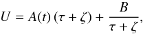 (25)with B = const, which is a
particular, spherical case in Paper I, Eq. (31).
(25)with B = const, which is a
particular, spherical case in Paper I, Eq. (31).
6. Conclusions
The conditions of consistency studied in Paper I proved that a finite mixture of stellar populations was able to describe the main features of the local velocity distribution without having to change the axisymmetry hypothesis. However, in the Galactic plane, single populations had velocity ellipsoids without vertex deviation, so that the apparent vertex deviation of the disc velocity distribution was the result of different radial and rotation mean motions of the populations. Now, as a corollary, we have investigated the same problem under point-axial symmetry, in order to see how it might improve the velocity distribution approximation.
For the point-axial symmetry case, the local kinematic features are similarly derived from a mixture of stellar populations, each one according to a quadratic velocity distribution in the peculiar velocities satisfying the BCE, with a common potential allowing for the populations to be kinematically independent. This means that the populations should differ not only in rotation, but also in radial and vertical mean motions. Under the point-axial hypothesis we should also expect single populations with velocity ellipsoids having non-null vertex deviation and non-vanishing tilt, as well as a point-axial mass distribution.
An important fact is that the potential must be axisymmetric in order to support a quadratic integral of motion for each population, which usually represents a stellar system in statistical equilibrium. That is, we assume that the stellar system has achieved relaxation and satisfies regularity conditions about the definition of the local standard of rest, continuity, and differentiability of its velocity, and that higher-order velocity moments exist. Although dissipative forces related to third and odd-order moments does not appear in the moment equations planned for a single population, they are indirectly connected with the assumption of the mixture model.
The first result we obtain is that the point-axial symmetry is, in a natural way, consistent with the flat velocity distribution of a disc population, by providing potentials not depending on the population parameter K4, which is responsible for non-isothermal velocity distributions. In axisymmetric systems, only a particular family of potentials is consistent with a flat velocity distribution, while in point-axial systems any potential always is.
We find two possible solutions depending on the separability of the potential:
-
(a)
The point-axial model admits a potential additively separablein cylindrical coordinates that is the harmonic potential. As in theaxisymmetric model, for a separable potential there is no need ofconditions of consistency in regard to a mixture distribution,since the potential only constrains the population parametersthrough the function A(t) (Paper I, Eq. (20)). For each population, the radial and vertical mean velocities can be different, and their velocity ellipsoids can have different orientations, including the both vertex deviation and tilt.
-
(b)
For a non-separable potential, the condition given by Eq. (24)provides nearly non-constrained population kinematics, by leading to a spherical and quasi-stationary potential. Then, the radial and the vertical mean velocities can differ among populations, although they are coupled, and they may produce an apparent vertex deviation of the whole velocity distribution. However, single population velocity ellipsoids have no vertex deviation in the Galactic plane and no tilt in their intersection with a meridional Galactic plane, similarly to the axisymmetric case.
In both of these cases, the potential for the point-axial model becomes a particular function of the potential for the axisymmetric model. The non-separable potential loses the dependency on the elevation angle, and the separable potential loses the non-harmonic term that they showed in Paper I (Eqs. (31) and (33), respectively).
We can check the foregoing cases according to the main local kinematic trends analysed in Paper I. Against option (a) is the evidence that there are halo stars near the Sun with no net rotation velocity for which the harmonic potential is not able to support their orbits. On the other hand, option (b) really provides a potential, Eq. (25), with a non-harmonic term, which may be associated with a repulsive force (if B> 0) produced by the outer dark matter halo, as discussed in Paper I. This allows stable orbits for stars with no net rotation. However, the potential forces the population velocity ellipsoids to point toward the Galactic centre, although, out of the Galactic plane, the ellipsoids may show some vertex deviation.
Then, according to the point-axial model, how can we explain that the thick disc and the halo ellipsoids have no vanishing tilt, as Casetti-Dinescu (2011), Carollo et al. (2010), Fuchs et al. (2009), Smith et al. (2009a), and Siebert et al. (2008) suggest? By assuming that the harmonic potential is not realistic, under the point-axial model we cannot explain it. Similarly, the point-axial model is unable to explain the trend of the moment μϖz for the thin disc population described by Pasetto et al. (2012b), which was only possible under a separable potential, as discussed in Paper I.
Conversely, if the thick disc and the halo ellipsoids actually have a non-vanishing tilt, the axisymmetric model is capable of making a reasonable approach to the local features of the local velocity distribution. Therefore, we must conclude that the velocity distribution in the solar neighbourhood reflects a basically axisymmetric Galaxy.
Nevertheless, we should not discard the fact that some of the stellar samples used to describe the thick disc and the halo could have stars that were not sufficiently mixed to produce well defined velocity ellipsoids, or were contaminated by disc stars, as Smith et al. (2009a) suggest. If newer and more accurate analyses yielded non-tilted velocity ellipsoids for the thick disc and the halo, both models would be capable of describing the local velocity distribution from a non-separable potential, which, in all cases, would provide an axisymmetric velocity distribution in the Galactic plane.
However, for the stellar density, point-axial symmetry matters. We may assume a
Schwarzschild velocity distribution without loss of generality to discuss the shape of mass
distribution. In that case, the stellar density is  (Eq.
(40) in Appendix A.2 in Paper I) and depends on the angle through K4(θ). Leaving aside the
simple and unrealistic case of a separable and harmonic potential, for the non-separable
potential with k ≡
K1 = k3, Eq.
(25)is a particular case of Eq. (23)with
(Eq.
(40) in Appendix A.2 in Paper I) and depends on the angle through K4(θ). Leaving aside the
simple and unrealistic case of a separable and harmonic potential, for the non-separable
potential with k ≡
K1 = k3, Eq.
(25)is a particular case of Eq. (23)with 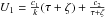 .
The function σ
involved in the stellar density satisfies
.
The function σ
involved in the stellar density satisfies 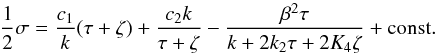 (26)For ζ = 0, σ does not depend on
θ. However,
for ζ = 0, we
have
(26)For ζ = 0, σ does not depend on
θ. However,
for ζ = 0, we
have 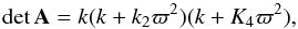 (27)so that, in the
Galactic plane, the stellar density N depends on θ. This dependency of the
mass distribution on the angle is balanced out by the velocity distribution, which also
depends on θ,
while the potential maintains the axisymmetry. This is the only basic feature that the
point-axial model adds to the axisymmetric model. While, in the Galactic plane, for the
velocity distribution, according to Eqs. (3) and (27), the tensor element Azz and detA, which depend on
θ, lead to
moments μϖϖ,μzz
also depending on the angle, although each population component is unable to provide a
non-vanishing moment μϖθ. Thus, similarly to
the axisymmetric case, for ellipsoidal velocity distributions under a non-separable
potential, the apparent vertex deviation of the velocity distribution is a consequence of
the coexistence of two or more populations with different radial and rotation mean
velocities.
(27)so that, in the
Galactic plane, the stellar density N depends on θ. This dependency of the
mass distribution on the angle is balanced out by the velocity distribution, which also
depends on θ,
while the potential maintains the axisymmetry. This is the only basic feature that the
point-axial model adds to the axisymmetric model. While, in the Galactic plane, for the
velocity distribution, according to Eqs. (3) and (27), the tensor element Azz and detA, which depend on
θ, lead to
moments μϖϖ,μzz
also depending on the angle, although each population component is unable to provide a
non-vanishing moment μϖθ. Thus, similarly to
the axisymmetric case, for ellipsoidal velocity distributions under a non-separable
potential, the apparent vertex deviation of the velocity distribution is a consequence of
the coexistence of two or more populations with different radial and rotation mean
velocities.
Then, a point-axisymmetric stellar system would, in principle, be able to show a triaxial or bar-like structure in any of the population’s mass distributions. It would be a matter of time that, for the specific population, the rotation curve could transform a bar-like into a spiral-like structure. In that situation, the point-axial model would have the ability to describe a point-axial mass distribution, while the axial model would not. However, we note that the degenerate case of a rigid rotating bar, with k2 = 0, which was the only remaining case that could admit, a priori, a non-cylindrical potential as a solution of Eq. (9), cannot coexist with three-dimensional ellipsoidal velocity distributions under a common differentiable point-axial potential. Hence, any phase mixing process involving a rigid rotating bar with a non-cilyndrical potential must be considered as a state previous to statistical equilibrium, which is not associated with stellar populations having ellipsoidal velocity distributions, even with point-axial symmetry.
Appendix
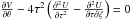
The first three partial differential equations for the potential, obtained by taking the
curl in Eq. (6), are ![Mathematical equation: \begin{equation} \label{tot1} \begin{array}{l} 8 K_4\tau \left[2 \left( \frac{\partial U}{\partial \tau}-\frac{\partial U}{\partial \zeta} \right)+ \tau \frac{\partial}{\partial\tau} \left( \frac{\partial U}{\partial \tau}-\frac{\partial U}{\partial \zeta} \right) +\zeta \frac{\partial}{\partial \zeta} \left( \frac{\partial U}{\partial \tau}-\frac{\partial U}{\partial \zeta} \right)\right] \\[2mm] +4 \tau (K_1-k_3) \frac{\partial^2 U}{\partial \tau \partial \zeta}+ 2 K'_4 \frac{\partial}{\partial \theta}\left( \tau \frac{\partial U}{\partial \tau}+ U +\zeta \frac{\partial U}{\partial \zeta} \right)+ K'_1 \frac{\partial^2 U}{\partial \theta \partial \zeta}= 0, \end{array} \end{equation}](/articles/aa/full_html/2014/07/aa23813-14/aa23813-14-eq140.png) (28)where
a common factor proportional to
(28)where
a common factor proportional to  was simplified;
 ![Mathematical equation: \begin{equation} \label{tot2} \begin{array}{l} 4 K'_4 \tau \left[2 \left( \frac{\partial U}{\partial \tau}-\frac{\partial U}{\partial \zeta} \right)+ \zeta \frac{\partial}{\partial \zeta}\left( \frac{\partial U}{\partial \tau}-\frac{\partial U}{\partial \zeta} \right)\right]+ 2 K'_1 \tau \frac{\partial^2 U}{\partial \tau \partial \zeta}\\[2mm] +4 K'_4 \tau \frac{\partial^2 U}{\partial \theta^2} + 2(3K^*_4-K_4)\frac{\partial U}{\partial \theta}+ 4 K_4 \tau \frac{\partial^2 U}{\partial \theta \partial\tau}\\[2mm] -\left[2(k_3-K^*_1)+4(K_4-k_2)\tau-4 K^*_4 \zeta\right] \frac{\partial^2 U}{\partial \theta\zeta} =0, \end{array} \end{equation}](/articles/aa/full_html/2014/07/aa23813-14/aa23813-14-eq142.png) (29)where
a common factor proportional to
was simplified; and
(29)where
a common factor proportional to
was simplified; and ![Mathematical equation: \begin{equation} \label{tot3} \begin{array}{l} 4\tau^2\left[ 2 K'_4 \zeta \frac{\partial}{\partial \tau}\left( \frac{\partial U}{\partial \tau}-\frac{\partial U}{\partial \zeta} \right) + K'_1 \frac{\partial^2 U}{\partial \tau^2}\right]- (K'_1+2K'_4\zeta) \frac{\partial^2 U}{\partial \theta^2} \\[2mm] +8K_4\tau\zeta \frac{\partial^2 U}{\partial \theta\partial\zeta}+ 4\tau[2k_2\tau-(K_1-K_1^*)-2(K_4-K_4^*)\zeta] \frac{\partial^2 U}{\partial \theta\partial \tau}\\[2mm] +2\left[4k_2\tau+(K_1-K_1^*)+2(K_4-K_4^*)\zeta\right] \frac{\partial U}{\partial \theta} =8 \dot \beta \tau . \end{array} \end{equation}](/articles/aa/full_html/2014/07/aa23813-14/aa23813-14-eq143.png) (30)Those
equations which were proportional to
become null at the Galactic plane.
(30)Those
equations which were proportional to
become null at the Galactic plane.
The remaining three equations, which are obtained by taking the gradient in Eq. (7)and the time derivative in Eq. (6), are ![Mathematical equation: \begin{equation} \label{tot4} \begin{array}{l} 2 K_4 \zeta \frac{\partial}{\partial t}\left( \frac{\partial U}{\partial \tau}-\frac{\partial U}{\partial \zeta} \right)\\[2mm] +\dot{K_1} \tau \frac{\partial^2 U}{\partial \tau^2}+ K_1 \frac{\partial^2 U}{\partial t \partial \tau} + 2 \dot{K_1} \frac{\partial U}{\partial \tau} +\frac12 \dddot{K_1} + \dot{k_3} \zeta \frac{\partial^2 U}{\partial \tau \partial \zeta}\\[2mm] +\frac{1}{4\tau} \left[(\dot K'_1-4\beta)\tau \frac{\partial^2 U}{\partial \theta\partial \tau}+ (K'_1+2 K'_4\zeta) \frac{\partial^2 U}{\partial \theta \partial t}+ (\dot K'_1+2\dot K'_4\zeta) \frac{\partial U}{\partial \theta}\right]=0; \end{array} \end{equation}](/articles/aa/full_html/2014/07/aa23813-14/aa23813-14-eq144.png) (31)
(31)![Mathematical equation: \begin{equation} \label{tot5} \begin{array}{l} 2 K_4 \tau \frac{\partial}{\partial t}\left( \frac{\partial U}{\partial \zeta}-\frac{\partial U}{\partial \tau} \right) \\[2mm] +\dot{k_3} \zeta \frac{\partial^2 U}{\partial \zeta^2}+ k_3 \frac{\partial^2 U}{\partial t \partial \zeta} + 2 \dot{k_3} \frac{\partial U}{\partial \zeta} +\frac12 \dddot{k_3} + \dot{K_1} \tau \frac{\partial^2 U}{\partial \zeta \partial \tau}\\[2mm] +(\dot K'_1-4\beta) \frac{\partial^2 U}{\partial \theta\partial \zeta} -\frac14 K'_4 \frac{\partial^2 U}{\partial \theta \partial t} =0; \end{array} \end{equation}](/articles/aa/full_html/2014/07/aa23813-14/aa23813-14-eq145.png) (32)in
the last one, a common factor
was also simplified; and
(32)in
the last one, a common factor
was also simplified; and ![Mathematical equation: \begin{equation} \label{tot6} \begin{array}{l} \tau\left[2 K'_4 \zeta \frac{\partial}{\partial t}\left( \frac{\partial U}{\partial \tau}-\frac{\partial U}{\partial \zeta} \right)+ K'_1 \frac{\partial^2 U}{\partial t \partial \tau} + 2 \dot{K'_1} \frac{\partial U}{\partial \tau} +\frac12 \dddot{K'_1}\right]\\[2mm] +\dot K_1 \tau \frac{\partial^2 U}{\partial \theta\partial \tau}+ \frac14 (\dot K'_1-4\beta) \frac{\partial^2 U}{\partial \theta^2}+ \dot{k_3} \zeta \frac{\partial^2 U}{\partial \theta\partial \zeta}\\[2mm] +(K^*_1+2 k_2 \tau+ 2 K_4\zeta) \frac{\partial^2 U}{\partial \theta \partial t}+ \frac14 (\dot K''_1+4K^*_1) \frac{\partial U}{\partial \theta} =2 \ddot \beta \tau. \end{array} \end{equation}](/articles/aa/full_html/2014/07/aa23813-14/aa23813-14-eq146.png) (33)These
equations complete the first set of three equations given by Sanz-Subirana (1987). They may be simplified by assuming that the
parameter β is
constant, which was actually derived by this author in solving them for the separable
potential case, and by Juan-Zornoza (1995) for the
general case. This fact is not relevant for our purpose.
(33)These
equations complete the first set of three equations given by Sanz-Subirana (1987). They may be simplified by assuming that the
parameter β is
constant, which was actually derived by this author in solving them for the separable
potential case, and by Juan-Zornoza (1995) for the
general case. This fact is not relevant for our purpose.
In cylindrical coordinates (ϖ,θ,z) the stationary potential consistent with a
quadratic velocity distribution is  , with A constant and
V an
arbitrary function that does not depend on time. When A is a time dependent
function, the potential was called quasi-stationary in Paper I.
, with A constant and
V an
arbitrary function that does not depend on time. When A is a time dependent
function, the potential was called quasi-stationary in Paper I.
In Paper I, the asymptotic case K4 → 0 was called flat velocity distribution, which, according to Chandrasekhar (1962), applies to the velocity distribution of an ideal disc. Although a disc stellar population can be approximated by this model, the other populations have a velocity distribution that must depend on z. Therefore, in general we must assume that K4 is non-null.
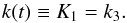
As pointed out in Paper I, the second-order central velocity moments satisfy
μ ∝
A-1. In the Galactic plane, from Eq. (3), we get  .
.
Although we assume that the velocity distribution is π-periodic, we cannot discard that part of the potential function could still admit a 2π-periodic solution.
In this case, we first prove that, if  , the equation
 , with the variables
x = lnτ,y =
ζ/τ, provides a
solution proportional to an exponential function on the argument x + θ,
which is not periodic and, hence, unacceptable. We then verify that the remaining terms of
Eq. (8)do not vanish, otherwise, its
solution, which takes the general form
, with the variables
x = lnτ,y =
ζ/τ, provides a
solution proportional to an exponential function on the argument x + θ,
which is not periodic and, hence, unacceptable. We then verify that the remaining terms of
Eq. (8)do not vanish, otherwise, its
solution, which takes the general form 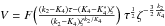 ,
has discontinuities either at ζ = 0 or at points satisfying
,
has discontinuities either at ζ = 0 or at points satisfying
 .
.
Similarly, by reasoning in regard to a population mixture, the potential is independent from the population parameters only if both parts are null separately.
Acknowledgments
The author wishes to thank the anonymous referee for his/her useful comments that have contributed to improving this paper.
References
- Camm, G. L. 1941, MNRAS, 101, 195 [NASA ADS] [CrossRef] [Google Scholar]
- Carollo, D., Beers, T. C., Chiba, M., et al. 2010, ApJ, 712, 692 [NASA ADS] [CrossRef] [Google Scholar]
- Casetti-Dinescu, D. I., Girard, T. M., Korchagin, V. I., & van Altena, W. F. 2011, ApJ, 728,7 [NASA ADS] [CrossRef] [Google Scholar]
- Chandrasekhar, S. 1960, Principles of Stellar Dynamics (New York: Dover Publications Inc.) [Google Scholar]
- Cubarsi, R. 2007, MNRAS, 207, 380 [Google Scholar]
- Cubarsi, R. 2010, A&A, 522, A30 [NASA ADS] [CrossRef] [EDP Sciences] [Google Scholar]
- Cubarsi, R. 2014, A&A, 561, A141 [NASA ADS] [CrossRef] [EDP Sciences] [Google Scholar]
- Fuchs, B., Dettbarn, C., & Rix, H-W. 2009, AJ, 137, 4149 [NASA ADS] [CrossRef] [Google Scholar]
- Juan-Zornoza, J. M. 1995, Ph.D. Thesis (ISBN: 844750767-X), University of Barcelona [Google Scholar]
- Juan-Zornoza, J. M., & Sanz-Subirana, J. 1991, Ap&SS, 185, 95 [NASA ADS] [CrossRef] [Google Scholar]
- Juan-Zornoza, J. M., Sanz-Subirana, J., & Cubarsi, R. 1990, Ap&SS, 170, 343 [NASA ADS] [CrossRef] [Google Scholar]
- MoniBidin, C., Carraro, G., & Méndez, R. A. 2012, ApJ, 747, 101 [NASA ADS] [CrossRef] [Google Scholar]
- Pasetto, S., Grebel, E. K., Zwitter, T., et al. 2012a, A&A, 547, A70 [NASA ADS] [CrossRef] [EDP Sciences] [Google Scholar]
- Pasetto, S., Grebel, E. K., Zwitter, T., et al. 2012b, A&A, 547, A71 [NASA ADS] [CrossRef] [EDP Sciences] [Google Scholar]
- Sanz-Subirana, J. 1987, Ph.D. Thesis (ISBN: 8475282326), University of Barcelona [Google Scholar]
- Siebert, A., Bienaymé, O., Binney, J., et al. 2008, MNRAS, 391, 793 [NASA ADS] [CrossRef] [Google Scholar]
- Siebert, A., Williams, M. E. K., Siviero, A., et al. 2011, AJ, 141, 187 [NASA ADS] [CrossRef] [Google Scholar]
- Smith, M. C., Evans, N. W., An, J. H. 2009a, ApJ, 698, 1110 [NASA ADS] [CrossRef] [Google Scholar]
- Smith, M. C., Evans, N. W., Belokurov, V., et al. 2009b, MNRAS, 399, 1223 [NASA ADS] [CrossRef] [Google Scholar]
- Steinmetz, M. 2012, Astron. Nachr., 333, 523 [NASA ADS] [CrossRef] [Google Scholar]
- Steinmetz, M., Zwitter, T., Siebert, A., et al. 2006, AJ, 132, 1645 [NASA ADS] [CrossRef] [Google Scholar]
- Vandervoort, P. O. 1979, ApJ, 232, 91 [NASA ADS] [CrossRef] [Google Scholar]
- Zwitter, T., Siebert, A., Munari, U., et al. 2008, AJ, 136, 421 [NASA ADS] [CrossRef] [Google Scholar]
Current usage metrics show cumulative count of Article Views (full-text article views including HTML views, PDF and ePub downloads, according to the available data) and Abstracts Views on Vision4Press platform.
Data correspond to usage on the plateform after 2015. The current usage metrics is available 48-96 hours after online publication and is updated daily on week days.
Initial download of the metrics may take a while.