| Issue |
A&A
Volume 567, July 2014
|
|
|---|---|---|
| Article Number | A18 | |
| Number of page(s) | 7 | |
| Section | Atomic, molecular, and nuclear data | |
| DOI | https://doi.org/10.1051/0004-6361/201423729 | |
| Published online | 04 July 2014 | |
Atomic data for astrophysics: Ni XV⋆
1
DAMTP, Centre for Mathematical Sciences, Wilberforce Road,
Cambridge
CB3 0WA,
UK
e-mail:
g.del-zanna@damtp.cam.ac.uk
2
Department of Physics and Astronomy, University College
London, Gower
Street, London
WC1E 6BT,
UK
Received: 28 February 2014
Accepted: 30 April 2014
We present the first R-matrix scattering calculation for electron collisional excitation of Ni xv. The large-scale target includes configurations up to n = 4. The calculations were carried out using the intermediate-coupling frame transformation method. Significant enhancements in the collision strengths, compared to previous distorted-wave (DW) calculations, are found for several cases, in particular the forbidden lines within the ground configuration and the 3s2 3p 4s levels. We provide a complete set of rates and a list of strongest lines that are observable in astrophysical plasmas. Previous identifications are reviewed, and a few new ones suggested. The new data can be used to accurately measure electron densities for high-temperature (3 MK) plasmas, and the nickel abundance.
Key words: atomic data / line: identification / techniques: spectroscopic / Sun: corona
The full dataset (energies, transition probabilities and rates) is available from our APAP website http://www.apap-network.org, and also at the CDS via anonymous ftp to cdsarc.u-strasbg.fr (130.79.128.5) or via http://cdsarc.u-strasbg.fr/viz-bin/qcat?J/A+A/567/A18
© ESO, 2014
1. Introduction
Ni xv produces strong decays from the 3s 3p3 and 3s2 3p 3d configurations in the extreme ultraviolet (EUV) region of the spectrum (Behring et al. 1972), most of which were identified by Fawcett & Hayes (1972) and Fawcett & Hatter (1980). Some of these lines are useful density and abundance diagnostics for high-temperature (3 MK) plasmas, such as those of solar active region cores (Del Zanna 2013b).
Ni xv also produces two important forbidden lines (within the n = 3) in the visible region of the spectrum, identified by Edlén (1942), and often observed during total solar eclipses (e.g. Aly et al. 1962; Jefferies et al. 1971; Fisher & Pope 1971; Mason 1973). They are also potentially very useful density diagnostics, like the well known isoelectronic Fe xiii infrared lines. Ni xv soft X-ray transitions from the n = 4 levels have also been observed in the laboratory (Fawcett et al. 1972; Kastner et al. 1978).
Landi & Bhatia (2012) published the first complete scattering calculation for this ion. They used the Flexible Atomic Code (Gu 2004) and the distorted-wave (DW) approximation to calculate collision strengths to the 3s2 3p2, 3s 3p3, 3s2 3p 3d, 3p4, 3s 3p2 3d, and 3s2 3p 4l (l = s, p, d, f) configurations.
Ni xv is isoelectronic with Fe xiii, for which we now have a fairly complete set of line identifications and atomic data. A complete review of the Fe xiii line identifications and wavelengths for the n = 3 levels was given in Del Zanna (2011), where a number of new energy levels were identified, using the Iron Project scattering calculations of Storey & Zeippen (2010). These authors performed an R-matrix calculation for the lowest 54 LS terms and 114 fine-structure levels within the n = 3 complex.
In Del Zanna & Storey (2013) we carried out a large-scale R-matrix (up to n = 4) scattering calculations for electron collisional excitation of Fe xiii. For the scattering close-coupling calculation, we retained 749 fine-structure levels arising from the first 331 LS terms. As found in previous similar work on Fe x (Del Zanna et al. 2012), the excitation rates to some of the states of the n = 4 configurations are significantly increased by resonances converging on other n = 4 states.
Our experience on the Fe xiii shows that the DW approximation significantly underestimates the collisions strengths, especially for the energetically lowest configurations. An R-matrix calculation for this ion was therefore needed, to improve on the Landi & Bhatia (2012) calculations. In Sect. 2 we outline the methods we adopted for the scattering calculations. In Sect. 3 we present our results and in Sect. 4 we reach our conclusions.
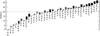 |
Fig. 1 Term energies of the target levels. The lowest 230 terms which produce levels having energies below the dashed line have been retained for the close-coupling expansion. |
2. Methods
The atomic structure calculations were carried out using the autostructure program (Badnell 2011), which originated from the superstructure program (Eissner et al. 1974). autostructure constructs target wavefunctions using radial wavefunctions calculated in a scaled Thomas-Fermi-Dirac statistical model potential with a set of scaling parameters. The program also provides radiative rates and infinite energy Born limits. These limits are particularly important from two aspects. First, they allow a consistency check of the collision strengths in the scaled Burgess & Tully (1992) domain (see also Burgess et al. 1997). Second, they are used in the interpolation of the collision strengths at high energies.
The R-matrix method used in the scattering calculation is described in Hummer et al. (1993) and Berrington et al. (1995). We performed the calculation in the inner region in LS coupling and included mass and Darwin relativistic energy corrections.
The outer region calculation used the intermediate-coupling frame transformation method (ICFT) described by Griffin et al. (1998), in which the transformation of the multi-channel quantum defect theory unphysical K-matrix to intermediate coupling uses the so-called term-coupling coefficients (TCCs) in conjunction with level energies.
Dipole-allowed transitions were topped-up to infinite partial wave using an intermediate coupling version of the Coulomb-Bethe method as described by Burgess (1974) while non-dipole-allowed transitions were topped up assuming that the collision strengths form a geometric progression in J (see Badnell & Griffin 2001).
The collision strengths were extended to high energies by interpolation using the appropriate high-energy limits in the Burgess & Tully (1992) scaled domain. The high-energy limits were calculated with autostructure for both optically-allowed (see Burgess et al. 1997) and non-dipole-allowed transitions (see Chidichimo et al. 2003).
We have also carried out Breit-Pauli DW calculations using the recent development of the autostructure code, described in detail in Badnell (2011).
The temperature-dependent effective collisions strength Υ(i − j) were calculated by assuming a Maxwellian electron distribution and linear integration with the final energy of the colliding electron.
3. Results
3.1. The scattering calculation
For our configuration basis we have chosen the complete set of 35 n = 3,4 configurations shown in Fig. 1 and listed in Table 1. They give rise to 944 LS terms and 2186 fine-structure levels. The scaling parameters λnl for the potentials in which the orbital functions are calculated are also given in Table 1.
Target electron configuration basis and orbital scaling parameters λnl.
In our n = 4 calculations for Fe xiii (Del Zanna & Storey 2013), we found very small differences in the collision strengths to the n = 3 levels, compared to the previous results of Storey & Zeippen (2010). This means that the main resonances affecting the n = 3 levels are from within the n = 3 complex. Since in this paper we are primarily interested in the n = 3 diagnostics, we have chosen for the close-coupling expansion of Ni xv a set of LS terms that is slightly reduced, compared to what we adopted for Fe xiii. The 483 fine-structure levels arising from the (energetically) lowest 230 LS terms were retained for the scattering calculation. They include all the spectroscopically important levels, up to n = 4, in particular those from the 3s2 3p 4l (l = s, p, d, f) configurations.
Level energies for Ni xv.
Table 2 presents a selection of fine-structure target level energies Et, compared to experimental energies Eexp. The experimental energies are mostly taken from the NIST compilation (Kramida et al. 2013), which in turn relied on the identifications mentioned in the introduction. We also suggest some new itentifications, as described below.
We note that the level 3s2 3p21S0 is not listed by NIST, but was identified by Feldman et al. (1998) from the 2–5 3s2 3p23P1–3s2 3p21S0 transition observed by SOHO SUMER at 1033.04 Å. A few 3s 3p3 levels were in principle identified by Trigueiros et al. (2006) (and also adopted by Landi & Bhatia 2012), however, a close inspection of their results (Table 2) shows a few problems. The energy suggested for the 3D3 (level 9), 335 562 cm-1, is at odds with the NIST one and those of the 3D1 and 3D2, so must be incorrect. The suggested energy for the 3P0 (level 10), 385 082 cm-1, is at odds with the energy of the 3P2, so it must also be incorrect. The energy of the 3P2 was listed as new, but was actually obtained by Fawcett & Hayes (1972). The only new energy listed by Trigueiros et al. (2006) that is correct is that of the 3P1 (level 11). Its value can be estimated quite accurately from the energy of the 3P2, and it is in agreement with the wavelength of the 3s2 3p23P0–3s 3p33P1 line, observed at 259.43 Å by Trigueiros et al. (2006). We can confirm independently this identification because we observe the 3s2 3p23P1–3s 3p33P1 line with Hinode EIS at 269.87 Å (see Del Zanna 2012b). The energies of the few n = 4 levels are discussed below.
A set of “best” energies Eb was obtained with a linear fit between the Eexp and Et values. The Eb values were used (whenever the experimental energies Eexp were not available) within the R-matrix calculation to obtain a better position of the resonance thresholds. The experimental energies Eexp and the “best” energies Eb were also used to calculate the transition probabilities, which was done with a separate autostructure calculation.
The expansion of each scattered electron partial wave was done over a basis of 18 functions within the R-matrix boundary and the partial wave expansion extended to a maximum total orbital angular momentum quantum number of L = 16. This produces reliable collision strengths up to about 80 Ryd.
The outer region calculation includes exchange up to a total angular momentum quantum number J = 27/2. We have supplemented the exchange contributions with a non-exchange calculation extending from J = 29/2 to J = 75/2. The outer region exchange calculation was performed in a number of stages. A coarse energy mesh was chosen above all resonances. The resonance region itself was calculated with 6400 points.
We calculated the thermally-averaged collision strengths, Υ, which are, as we expected, significantly enhanced compared to the DW results of Landi & Bhatia (2012), for several important transitions. A few examples are given in Fig. 2. The enhancements mainly affect the transitions between levels of the ground configuration. For strong dipole-allowed transitions the effects of the resonances are expected to be small, and indeed we find excellent agreement between our thermally averaged collision strengths and those of Landi & Bhatia (2012), as illustrated by the 1–14 and 1–20 transitions in Fig. 2.
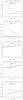 |
Fig. 2 Thermally averaged collision strengths for a selection of transitions (see text). The DW results are from Landi & Bhatia (2012). |
List of the strongest Ni xv lines.
3.2. Comparison to observations
We have constructed an ion population model with the new R-matrix collision strengths, complemented with a set of A-values calculated separately with exactly the same configuration basis as the scattering target, but with the experimental and best energies. We then calculated line intensities and looked at how levels are populated at log Ne [cm-3] = 9 (a typical solar active region density) and log Te [K] = 6.4, the temperature of maximum ion abundance for Ni xv in ionization equilibrium. The brightest lines are listed in Table 3.
The strongest EUV line, at 176.74 Å, is well visible with the Hinode EIS instrument, and indeed has been used e.g. in Del Zanna (2013b) to measure the nickel abundance in hot active region loops, relative to other elements. This line, in quiet Sun coronal observations, is blended with an Fe vii line (Del Zanna 2009).
The density-sensitive line at 179.27 Å (which is actually a self-blend with a weaker transition) is very close in wavelength to the strongest line at 176.74 Å. These two lines are therefore an excellent density diagnostic, like the widely used Fe xiii 202, 203.8 Å lines. One problem is that these lines fall in a spectral region where the Hinode EIS sensitivity decreases very rapidly, hence long exposures are needed. We use here a spectrum of an active region core, observed on 2010 October 26, and discussed in Del Zanna (2013b). Parts of this spectrum are shown in Fig. 3.
The other Ni xv EUV lines observed by EIS are difficult to observe because they fall very close to other lines. The 184.88 Å is measurable, but it is in the red wing of a strong Fe xi line. The 185.69 Å line is blended with an unidentified line, and the 189.24 Å is also in the red wing of a much stronger line (for a discussion on identifications of EIS coronal lines see Del Zanna 2009, 2012b).
We use the new in-flight EIS radiometric calibration described in Del Zanna (2013a). This has significant differences compared to the ground calibration.
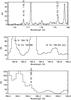 |
Fig. 3 Hinode EIS spectrum of a hot active region core at the wavelengths where some of the main EUV Ni xv lines are observed. |
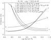 |
Fig. 4 Emissivity ratio curves for the lines observed by Hinode EIS in a hot active region core. The intensities Iob are in phot cm-2 s-1 arcsec-2. |
We show in Fig. 4 the “emissivity ratio” curve  (1)for each line as a function of the electron density Ne. Iob is the observed intensity of the line, Nj(Ne,Te) is the population of the upper level j relative to the total number density of the ion, calculated at a fixed temperature Te. Aji is the spontaneous radiative transition probability, and C is a scaling constant. This constant is the same for all the lines, and its value is 1.25 × 10¹⁰. This value was chosen so that the emissivity ratios are near unity, to visually estimate, from the spread in the curves, the relative agreement between observed and predicted intensities for all the lines. In fact, if agreement between experimental and theoretical intensities is present, all lines should be closely spaced. If the plasma is nearly isodensity, all curves should cross at one point, giving the line-of-sight averaged density. The emissivity ratio curves are useful to see at once the density sensitivity of the different emission lines, but are equivalent to the usual single line ratio plots, where the theoretical ratio of two emission lines is plotted as a function of density. The emissivity ratio curves in Fig. 4 are calculated at log Te[K] = 6.4, the temperature of maximum ion abundance in ionization equilibrium, i.e. the temperature where, in normal coronal conditions, the Ni xv lines are formed.
Figure 4 shows an excellent agreement between predicted and observed intensities for all the lines, providing a density of about log Ne = 9.5, typical of active region cores, with the exception of the 269.87, which is brighter than predicted. There is also a small (20%) discrepancy in a branching ratio, between the 2–19 (line No. 4) and the 3–19 (line No. 5). However, these two lines are weak and close to stronger lines (cf. Fig. 3), so their observed intensity is difficult to estimate accurately. Finally, we point out that Ni xv has various other density diagnostics in the EUV (not observed by Hinode EIS), such as the 311.8 (strongly blended) and 298.1 Å lines, as discussed by Landi & Bhatia (2012).
3.2.1. Optical forbidden lines
Ni xv also produces several forbidden lines in the UV and visible part of the spectrum, as shown in Table 3.
The main visible forbidden lines are observed at 6702 and 8024 Å (air wavelengths), and are excellent density diagnostics, although they are significantly affected by photoexcitation, as already pointed out by Landi & Bhatia (2012), and as shown in Fig. 5. Clearly, any density measurement from these lines needs to take carefully into account photoexcitation and line-of-sight integration. The quiet Sun eclipse measurements of Fisher & Pope (1971) are consistent with an electron density of log Ne [cm-3] = 8, slightly lower than the density obtained from the stronger Fe xiii forbidden lines (log Ne [cm-3] = 8.4), which were observed simultaneously. The difference in electron density might be real, considering that Ni xv is formed at higher temperatures than Fe xiii.
It is interesting to notice the relatively small difference in the ratio of these two lines, compared to the ratio calculated with the DW rates from Landi & Bhatia (2012), despite the large differences in the collision strengths from the ground state, between the DW and the R-matrix calculations. This occurs because the levels of the ground configuration are mainly populated by cascading.
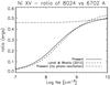 |
Fig. 5 Theoretical ratio of the main two visible forbidden lines from Ni xv, without photoexcitation (dot-dashed line) and with photoexcitation included, for a distance of 1.03 solar radii from Sun centre and a black-body photospheric spectrum at 6000 K. |
3.2.2. The soft X-ray lines
As in the case of the iron ions, soft X-ray transitions for Ni xv were identified in the laboratory, mostly by B.C. Fawcett. In Fawcett et al. (1972), he identified a few lines originating from the 3s2 3p 4s, 3s2 3p 4d, and 3s2 3p 4f. Later, Kastner et al. (1978) identified a few more decays from the 3s2 3p 4d, and 3s2 3p 4f configurations, although most of them had question marks. As in the case of Fe xiii and the other iron ions, the strongest soft X-ray transitions for Ni xv in typical solar/astrophysical conditions were not identified/observed in the laboratory, as shown in Table 3. The relative differences between observed and predicted wavelengths for the few known transitions is very small, so we can predict the wavelengths of the unidentified transitions quite accurately.
The Ni xv soft X-ray lines are intrinsically weaker than the iron lines, so only the few brightest ones should be observable. The brightest is a decay from a core-excited state, the 7−376 3s 3p33D1–3s 3p2 4s 3P0 transition. We identified these types of transitions for the first time for Fe x in Del Zanna et al. (2012) and for Fe xi, Fe xii, Fe xiii, and Fe xiv in Del Zanna (2012a), using an excellent soft X-ray spectrum obtained during an M1-class flare from a sounding rocket flight (Acton et al. 1985, hereafter A85). The spectral resolution was excellent, clearly resolving lines only 0.04 Å apart. The radiometric calibration was also very good. The predicted wavelength of the 7–376 line is 59.37 Å. There is a strong line at 59.59 Å in the A85 spectrum, and listed as a blend. The benchmark of the Fe xiv soft X-ray lines showed that less than 50% of the intensity of the line is due to Fe xiv (see Fig. 6 in Del Zanna 2012a), hence we identify the 7–376 with the 59.59 Å line.
The second strongest transition is the 20–439 3s2 3p 3d 3P1–3s2 3p 4f 3F2, with a theoretical wavelength of 62.88 Å. There are few lines in the A85 spectrum around the predicted wavelength. The benchmark carried out in Del Zanna (2012a) suggest that one option is that this line is blended with Fe xiii at 62.98 Å, which is in fact listed as blended in A85. Another option is the unidentified line at 63.57 Å, which results in a difference between predicted and observed energy for 3s2 3p 4f 3F2 of 25 433 cm-1, much closer to the energy difference for the only 4f level (26 751 cm-1), identified by Kastner et al. (1978). We opt for the second choice.
The next strong transitions are two decays from 3s2 3p 4p 3P0, level 328. We note that transitions from the 3s2 3p 4p levels were not identified previously. One option would be that the 7–328 transition is the line observed by A85 at 65.60 Å. Acton et al. identified this line as being due to Mg ix, however, the benchmark carried out in Del Zanna (2012a) indicates that Mg ix should be weak. This identification is excluded because the other decay (the 20–328) would then be expected at 77.28 Å, where A85 does not list any lines. We tentatively identify the 7–328 transition with the unidentified line observed by A85 at 65.90 Å, which would predict the other decay (20–328) at 77.70 Å. There is indeed a line at 77.73 Å listed by A85 as blended. The listed intensity is, however, in agreement with the predicted intensity from a Mg ix line (Del Zanna 2012a). We assume that the intensity provided by A85 refers to the main transition (Mg ix), and does not include the weaker Ni xv line. With this tentative identification, the difference between observed and predicted energy for the 3s2 3p 4p 3P0 level is 14 668 cm-1, in close agreement with the energy difference for the well-established 3s2 3p 4s levels. Further measurements, preferably in the laboratory, will be needed to confirm or rule out these tentative identifications.
Finally, comparing the intensities of the soft X-ray lines we have obtained with those obtained with the DW calculations (see Table 3), we can see quite a good agreement for those originating from the 3s2 3p 4p, 3s2 3p 4d, 3s2 3p 4f configurations but significant increases for those from 3s2 3p 4s. We have seen similar increases in Fe xiii, which are due to the effect of the resonances (Del Zanna & Storey 2013). For example, Fig. 2 (bottom plot) shows the effective collision strengths to the 3s2 3p 4s 3P1 level.
4. Conclusions
With the present work we have carried out the first R-matrix calculation for Ni xv. Significant differences with the previous
DW calculations of Landi & Bhatia (2012) are found, as expected, for a number of transitions. We have provided a complete set of rates and listed the strongest lines of this ion that are observable in astrophysical plasmas. We have assessed all the previous level and line identifications and suggested a few new ones. Our extended calculations and benchmarks for Fe xiii, and the few comparisons with observations discussed here, suggest that the present calculations are very accurate for lines from the n = 3 levels, which allow measurements of electron densities in high-temperature (3 MK) plasmas typical of solar active region cores, and of the nickel abundance.
Acknowledgments
The present work was funded by STFC (UK) through the University of Cambridge DAMTP astrophysics grant, and the University of Strathclyde UK APAP network grant ST/J000892/1.
References
- Acton, L. W., Bruner, M. E., Brown, W. A., et al. 1985, ApJ, 291, 865 (A85) [NASA ADS] [CrossRef] [Google Scholar]
- Aly, M. K., Evans, J. W., & Orrall, F. Q. 1962, ApJ, 136, 956 [NASA ADS] [CrossRef] [Google Scholar]
- Badnell, N. R. 2011, Comput. Phys. Commun., 182, 1528 [NASA ADS] [CrossRef] [Google Scholar]
- Badnell, N. R., & Griffin, D. C. 2001, J. Phys. B At. Mol. Phys., 34, 681 [NASA ADS] [CrossRef] [Google Scholar]
- Behring, W. E., Cohen, L., & Feldman, U. 1972, ApJ, 175, 493 [NASA ADS] [CrossRef] [Google Scholar]
- Berrington, K. A., Eissner, W. B., & Norrington, P. H. 1995, Comput. Phys. Commun., 92, 290 [NASA ADS] [CrossRef] [Google Scholar]
- Burgess, A. 1974, J. Phys. B At. Mol. Phys., 7, L364 [NASA ADS] [CrossRef] [Google Scholar]
- Burgess, A., & Tully, J. A. 1992, A&A, 254, 436 [NASA ADS] [Google Scholar]
- Burgess, A., Chidichimo, M. C., & Tully, J. A. 1997, J. Phys. B At. Mol. Phys., 30, 33 [NASA ADS] [CrossRef] [Google Scholar]
- Chidichimo, M. C., Badnell, N. R., & Tully, J. A. 2003, A&A, 401, 1177 [NASA ADS] [CrossRef] [EDP Sciences] [Google Scholar]
- Del Zanna, G. 2009, A&A, 508, 501 [NASA ADS] [CrossRef] [EDP Sciences] [Google Scholar]
- Del Zanna, G. 2011, A&A, 533, A12 [NASA ADS] [CrossRef] [EDP Sciences] [Google Scholar]
- Del Zanna, G. 2012a, A&A, 546, A97 [NASA ADS] [CrossRef] [EDP Sciences] [Google Scholar]
- Del Zanna, G. 2012b, A&A, 537, A38 [NASA ADS] [CrossRef] [EDP Sciences] [Google Scholar]
- Del Zanna, G. 2013a, A&A, 555, A47 [NASA ADS] [CrossRef] [EDP Sciences] [Google Scholar]
- Del Zanna, G. 2013b, A&A, 558, A73 [NASA ADS] [CrossRef] [EDP Sciences] [Google Scholar]
- Del Zanna, G., & Storey, P. J. 2013, A&A, 549, A42 [NASA ADS] [CrossRef] [EDP Sciences] [Google Scholar]
- Del Zanna, G., Storey, P. J., Badnell, N. R., & Mason, H. E. 2012, A&A, 541, A90 [NASA ADS] [CrossRef] [EDP Sciences] [Google Scholar]
- Edlén, B. 1942, Z. Astrophys., 22, 30 [Google Scholar]
- Eissner, W., Jones, M., & Nussbaumer, H. 1974, Comput. Phys. Commun., 8, 270 [NASA ADS] [CrossRef] [Google Scholar]
- Fawcett, B. C., & Hatter, A. T. 1980, A&A, 84, 78 [NASA ADS] [Google Scholar]
- Fawcett, B. C., & Hayes, R. W. 1972, J. Phys. B At. Mol. Phys., 5, 366 [Google Scholar]
- Fawcett, B. C., Cowan, R. D., & Hayes, R. W. 1972, J. Phys. B At. Mol. Phys., 5, 2143 [NASA ADS] [CrossRef] [Google Scholar]
- Feldman, U., Curdt, W., Doschek, G. A., et al. 1998, ApJ, 503, 467 [NASA ADS] [CrossRef] [Google Scholar]
- Fisher, R., & Pope, T. 1971, Sol. Phys., 20, 389 [NASA ADS] [CrossRef] [Google Scholar]
- Griffin, D. C., Badnell, N. R., & Pindzola, M. S. 1998, J. Phys. B At. Mol. Phys., 31, 3713 [NASA ADS] [CrossRef] [Google Scholar]
- Gu, M. F. 2004, in AIP Conf. Ser. 730, eds. J. S. Cohen, D. P. Kilcrease, & S. Mazavet, 127 [Google Scholar]
- Hummer, D. G., Berrington, K. A., Eissner, W., et al. 1993, A&A, 279, 298 [NASA ADS] [Google Scholar]
- Jefferies, J. T., Orrall, F. Q., & Zirker, J. B. 1971, Sol. Phys., 16, 103 [NASA ADS] [CrossRef] [Google Scholar]
- Kastner, S. O., Swartz, M., Bhatia, A. K., & Lapides, J. 1978, J. Opt. Soc. Am., 68, 1558 [NASA ADS] [CrossRef] [Google Scholar]
- Kramida, A., Ralchenko, Y., & Reader, J. 2013, NIST Atomic Spectra Database (ver. 5.1), available at http://physics.nist.gov/asd [Google Scholar]
- Landi, E., & Bhatia, A. K. 2012, At. Data Nucl. Data Tables, 98, 862 [Google Scholar]
- Mason, H. E. 1973, Ph.D. Thesis, University of London, UK [Google Scholar]
- Storey, P. J., & Zeippen, C. J. 2010, A&A, 511, A78 [NASA ADS] [CrossRef] [EDP Sciences] [Google Scholar]
- Trigueiros, A. G., Borges, F. O., Cavalcanti, G. H., & Farias, E. E. 2006, J. Quant. Spectr. Rad. Transf., 97, 29 [NASA ADS] [CrossRef] [Google Scholar]
All Tables
All Figures
|
Fig. 1 Term energies of the target levels. The lowest 230 terms which produce levels having energies below the dashed line have been retained for the close-coupling expansion. |
| In the text | |
|
Fig. 2 Thermally averaged collision strengths for a selection of transitions (see text). The DW results are from Landi & Bhatia (2012). |
| In the text | |
|
Fig. 3 Hinode EIS spectrum of a hot active region core at the wavelengths where some of the main EUV Ni xv lines are observed. |
| In the text | |
|
Fig. 4 Emissivity ratio curves for the lines observed by Hinode EIS in a hot active region core. The intensities Iob are in phot cm-2 s-1 arcsec-2. |
| In the text | |
|
Fig. 5 Theoretical ratio of the main two visible forbidden lines from Ni xv, without photoexcitation (dot-dashed line) and with photoexcitation included, for a distance of 1.03 solar radii from Sun centre and a black-body photospheric spectrum at 6000 K. |
| In the text | |
Current usage metrics show cumulative count of Article Views (full-text article views including HTML views, PDF and ePub downloads, according to the available data) and Abstracts Views on Vision4Press platform.
Data correspond to usage on the plateform after 2015. The current usage metrics is available 48-96 hours after online publication and is updated daily on week days.
Initial download of the metrics may take a while.