| Issue |
A&A
Volume 567, July 2014
|
|
|---|---|---|
| Article Number | A133 | |
| Number of page(s) | 17 | |
| Section | Numerical methods and codes | |
| DOI | https://doi.org/10.1051/0004-6361/201323350 | |
| Published online | 29 July 2014 | |
Evolution of the habitable zone of low-mass stars
Detailed stellar models and analytical relationships for different masses and chemical compositions⋆
1
Dipartimento di Fisica “Enrico Fermi”Università di Pisa,
largo Pontecorvo 3,
56127
Pisa,
Italy
e-mail:
This email address is being protected from spambots. You need JavaScript enabled to view it.
2
INFN, Sezione di Pisa, Largo B. Pontecorvo 3, 56127, Italy
Received:
28
December
2013
Accepted:
23
May
2014
Abstract
Context. The habitability of an exoplanet is assessed by determining the times at which its orbit lies in the circumstellar habitable zone (HZ). This zone evolves with time following the stellar luminosity variation, which means that the time spent in the HZ depends on the evolution of the host star.
Aims. We study the temporal evolution of the HZ of low-mass stars – only due to stellar evolution – and evaluate the related uncertainties. These uncertainties are then compared with those due to the adoption of different climate models.
Methods. We computed stellar evolutionary tracks from the pre-main sequence phase to the helium flash at the red-giant branch tip for stars with masses in the range [0.70−1.10] M⊙, metallicity Z in the range [0.005−0.04], and various initial helium contents. By adopting a reference scenario for the HZ computations, we evaluated several characteristics of the HZ, such as the distance from the host star at which the habitability is longest, the duration of this habitability, the width of the zone for which the habitability lasts one half of the maximum, and the boundaries of the continuously habitable zone (CHZ) for which the habitability lasts at least 4 Gyr. We developed analytical models, accurate to the percent level or lower, which allowed to obtain these characteristics in dependence on the mass and the chemical composition of the host star.
Results. The metallicity of the host star plays a relevant role in determining the HZ. The importance of the initial helium content is evaluated here for the first time; it accounts for a variation of the CHZ boundaries as large as 30% and 10% in the inner and outer border. The computed analytical models allow the first systematic study of the variability of the CHZ boundaries that is caused by the uncertainty in the estimated values of mass and metallicity of the host star. An uncertainty range of about 30% in the inner boundary and 15% in the outer one were found. We also verified that these uncertainties are larger than that due to relying on recently revised climatic models, which leads to a CHZ boundary shift within ±5% with respect to those of our reference scenario. We made an on-line tool available that provides both HZ characteristics and interpolated stellar tracks.
Key words: stars: evolution / stars: low-mass / methods: statistical / astrobiology / planets and satellites: physical evolution / planet-star interactions
On-line habitable zone calculator and track interpolator are available at http://astro.df.unipi.it/stellar-models/HZ/. The C code is also available at the CDS via anonymous ftp to cdsarc.u-strasbg.fr (130.79.128.5) or via http://cdsarc.u-strasbg.fr/viz-bin/qcat?J/A+A/567/A133
© ESO, 2014
1. Introduction
In the light of our limited knowledge, the existence of life is strongly associated with the presence of liquid water. The habitable zone (HZ) is then defined as the range of distances from a star within which a planet may contain liquid water at its surface (see e.g. Hart 1978; Kasting et al. 1993; Underwood et al. 2003; Selsis et al. 2007; Pierrehumbert & Gaidos 2011; Kopparapu et al. 2013). Several potentially habitable planets are already reported in literature (see among others Udry et al. 2007; Pepe et al. 2011; Borucki et al. 2011, 2012; Anglada-Escudé et al. 2012; Barclay et al. 2013; Tuomi et al. 2013; Batista et al. 2014), and their number is expected to increase with time.
The position of the HZ around the host star is not immutable with time, because it, and its width, are influenced by different climatological, biogeochemical, geodynamical, and astrophysical processes (see e.g. Kasting et al. 1993; Forget 1998; Selsis et al. 2007; von Bloh et al. 2009; Kopparapu et al. 2013; Leconte et al. 2013a). Although it is expected that – following the advance in the understanding of the interaction of all these processes – complex HZ models will eventually account self-consistently for all these aspects, at present no such model is available.
In this paper we focus on the evolution of the position of the HZ boundaries due only to the luminosity change of the host star. As explained in detail in Sect. 2, we evaluate some relevant HZ characteristics and quantify the uncertainty that affects these estimates only originating from the stellar observational uncertainties. To set these uncertainties in context, we also compare these values to those caused by different approximations in the HZ computations.
While evaluating the stellar uncertainty contribution to the overall uncertainty budget is only a single aspect of a very complex problem, at present it represents one of the firmest parts from the point of view of both observation and theory. Concerning the former, the stellar observables, such as luminosity, effective temperature, and metallicity can be determined much more accurately than the planetary ones. Concerning the latter, stellar evolution theory is one of the most mature and tested in the astrophysical literature. Moreover, the stellar impact on the HZ evolution will remain an essential ingredient in the future as well, when a more complete approach will be developed.
We restrict our analysis to low-mass stars – [0.70−1.10] M⊙ – for a large set of metallicities Z – [0.005−0.04] – and initial helium abundances Y. For more massive stars a similar study is reported in Lopez et al. (2005) and Danchi & Lopez (2013).
To evaluate the boundaries of the HZ, we relied on effective stellar fluxes obtained by climate models (see Sect. 2). In our HZ reference scenario computations we also assumed a constant planetary albedo and adopted the equilibrium temperature – that is, the temperature of a planet in thermal equilibrium between the radiation absorbed from the star and that radiated into space – as the parameter defining the position of the HZ. Within this scenario, the temporal evolution of the temperature of a planet at a given distance from the host star only depends on the evolution of the stellar luminosity. The boundaries of the HZ will then evolve following the changes of the luminosity with time. A planet is considered habitable if its equilibrium temperature is within the range of the allowed temperature obtained by climate models.
At variance with the other works published in the literature, we also provide here analytical relations of the dependence on the stellar mass and chemical composition of several important HZ features, namely the distance from the host star at which the longest duration of habitability occurs, the duration of this longest habitability, the width of the zone for which the habitability lasts at least one half of the maximum, and the position of the inner and outer boundaries for which the habitability lasts at least 4 Gyr. These analytical models have three purposes. First, they allow a systematic study of the variability of the HZ boundaries position due to the uncertainty in the estimates of the host star mass and metallicity, which is still lacking in the literature. Second, they allow distinguishing the contribution of the various stellar characteristics to the temporal variation of the HZ. Third, after a HZ boundary scenario is chosen, these models show the high degree of accuracy that can be achieved by analytical relations based on linear models.
We provide an on-line tool that allows a) downloading a stellar track for the chosen mass and chemical composition and b) obtaining the HZ characteristics.
The structure of the paper is the following: in Sect. 2 we discuss the method and the assumptions employed to computate the edges of the HZ and provide details on the adopted stellar evolutionary code and on the grid of the computed models. The main results are reported in Sect. 3, while the analytical models are discussed in Sect. 4. In Sect. 5 we present a comparison of the results given in Sect. 3 with those obtained without the constant albedo assumption and using the models by Kopparapu et al. (2013; hereafter K13). Concluding remarks are presented in Sect. 6.
2. Methods
We assumed an Earth-mass planet with an H2O/CO2/N2 atmosphere. Other atmospheric compositions, such as H2 rich ones, would change our results, moving the outer HZ boundary farther from the host star (see e.g. Stevenson 1999; Pierrehumbert & Gaidos 2011). We did not consider this class of objects here.
The HZ boundaries can be computed by assuming a grey-body approximation in which the
radiative properties of the planet are only described by the albedo A. The temporal variation of
the HZ boundaries is then described by the relation  (1)where L(t)
/L⊙ is the stellar
luminosity in solar units, and Seff is the effective stellar flux defined
as the value required to maintain a given surface temperature and calculated by the climatic
model as the ratio of the outgoing flux and the incident stellar flux. The contribution of
the planetary albedo, which is evaluated as a function of the effective temperature of the
host star, is internally accounted for in the models. These Seff critical
values are determined for both a dense H2O atmosphere at the inner edge and a dense
CO2 atmosphere with
1 bar of N2 and one
earth gravity at the outer edge.
(1)where L(t)
/L⊙ is the stellar
luminosity in solar units, and Seff is the effective stellar flux defined
as the value required to maintain a given surface temperature and calculated by the climatic
model as the ratio of the outgoing flux and the incident stellar flux. The contribution of
the planetary albedo, which is evaluated as a function of the effective temperature of the
host star, is internally accounted for in the models. These Seff critical
values are determined for both a dense H2O atmosphere at the inner edge and a dense
CO2 atmosphere with
1 bar of N2 and one
earth gravity at the outer edge.
A common approach to the HZ distance computations is to assume a constant planetary albedo
(see e.g. Borucki et al. 2011; Batalha et al. 2013; Cantrell et al.
2013; Danchi & Lopez 2013). Under
this hypothesis, equating the stellar fluxes absorbed and radiated by the planet (see e.g.
Kaltenegger & Sasselov 2011, for details of
the computation), Eq. (1) can be rewritten as
 (2)where A is the Bond albedo,
σ is the
Stefan-Boltzmann constant, a the conversion factor between centimeters and
astronomic units, and Tp is the planet equilibrium temperature.
In this scenario, the inner (di) and outer (do) radii of the
HZ can be easily computed from Eq. (2) after
the albedo and the corresponding temperatures Ti and To are fixed. The
explicit link between effective stellar flux, albedo and equilibrium temperature is given by
(2)where A is the Bond albedo,
σ is the
Stefan-Boltzmann constant, a the conversion factor between centimeters and
astronomic units, and Tp is the planet equilibrium temperature.
In this scenario, the inner (di) and outer (do) radii of the
HZ can be easily computed from Eq. (2) after
the albedo and the corresponding temperatures Ti and To are fixed. The
explicit link between effective stellar flux, albedo and equilibrium temperature is given by
 (3)In the computation we
adopted Eq. (2) as reference scenario, using
the Earth’s average Bond albedo (de Pater & Lissauer
2001, i.e. 0.3) for A.
(3)In the computation we
adopted Eq. (2) as reference scenario, using
the Earth’s average Bond albedo (de Pater & Lissauer
2001, i.e. 0.3) for A.
Significant progress is made in climate modelling, due to the development of 3D models (see e.g. Leconte et al. 2013a,b), which have shown systematic biases between mean surface temperatures predicted by 1D and 3D simulations. As a consequence, the associated estimates of the position of the HZ boundaries are expected to change in the forthcoming years. Therefore, giving actual estimates of the HZ and HZ characteristics is not the main goal of this paper. Instead, we are interested in analysing the dependence of several chosen features of the HZ on stellar evolution and on the quantification of the related uncertainties. This differential effect is expected to be robust to a change of the boundary positions by improved climate models.
We assumed as equilibrium temperature of the inner boundary of the HZ Ti = 269 K (see e.g. Forget 1998; Lopez et al. 2005; Selsis et al. 2007; Danchi & Lopez 2013). As discussed in detail in Selsis et al. (2007), this limit is determined considering that if the surface temperature remains below the critical temperature of water (647 K), the thermal emission of an habitable planet cannot exceed the runaway greenhouse threshold, equivalent to the irradiance of a black-body at 270 K. A planet with an atmosphere with an equilibrium temperature above 270 K either has a surface temperature below 647 K, but without liquid water on its surface, or a considerable amount of water, but a surface temperature above 1400 K. In both cases the planet would be uninhabitable for life as we know it.
The definition of the outer boundary position is more complicated, since there is no well-accepted estimate for the lowest insulation compatible with stable liquid water under a dense CO2 atmosphere. To tackle this problem, we adopted a set of effective stellar fluxes from 0.4 to 0.2 (Forget & Pierrehumbert 1997; Forget 1998; Mischna et al. 2000). These values correspond to equilibrium temperatures of To = 203 K and To = 169 K, assuming an albedo of 0.3. The former is set by the lowest temperature at which the liquid-solid phase change of water can occur, which depends on the existence of a greenhouse effect from CO2 and H2O (see e.g. Kasting et al. 1993; Forget 1998). The latter is based on planetary atmosphere models that include CO2 ice clouds. Atmospheres with optically thick CO2 ice clouds with large particle radii can more easily maintain the surface of a planet above the freezing point of water (Forget & Pierrehumbert 1997; Mischna et al. 2000; Wordsworth et al. 2011).
The adopted values of the inner and the outer borders equilibrium temperatures and the albedo are the same of Danchi & Lopez (2013), since we are interested in a comparison of the overlapping results. This comparison will give information about the uncertainty due only to the adoption of a different set of stellar tracks in the HZ computations.
We defined as continuously habitable zone (CHZ) a HZ lasting longer than 4 Gyr. Other choices are possible and values from 1 to 5 Gyr are adopted in literature (see e.g. Schopf 1993; Turnbull & Tarter 2003; Buccino et al. 2006).
Although the approach described above is currently widely adopted, it has known limits. Its main shortcoming is the assumption of an albedo A independent of the spectrum of the incoming radiation. As a matter of fact, the Bond albedo is not a planetary characteristics alone, but it also depends on the spectral energy distribution of the host star (see e.g. the extensive discussion on Selsis et al. 2007; Kaltenegger & Sasselov 2011). Computations of HZ that do not assume a constant albedo are available in literature (e.g. Selsis et al. 2007; Kopparapu et al. 2013); but they strongly depend on the climatic models used for the planetary atmosphere, on its compositions, on the scheme of cloud coverage, and on the considered geoclimatic processes, which are related in a still unknown manner to the mass of the planet (see e.g. Selsis et al. 2007, for details on these problems). Since these factors controlling a planet surface temperature are not yet constrained either by observations or by self-consistent models (see Seager 2013, for a review), we preferred to adopt in this work the simple model of Eq. (2) as our reference scenario.
However, it is interesting to evaluate the effect on the results of excluding the constant albedo assumption. In Sect. 5 we compare the results of our reference scenario with those obtained using the revised climate model presented in K13, without assuming a constant albedo. A similar comparison is presented in Danchi & Lopez (2013) for more massive stars. The correction is based on the parametrisation given in Selsis et al. (2007). For the HZ characteristics considered here, the differences due to excluding the constant albedo assumption are of the order of a few percent.
Figure 16 of Danchi & Lopez (2013) clearly shows that the duration of habitability of main-sequence solar and super-solar metallicity stars are essentially unaffected by the refinements in the boundary positions. According to that figure, the changes only influence the case at metallicity Z = 0.001, which is below the range considered here. Table 3 of the quoted paper shows that this statement also holds for the CHZ boundaries.
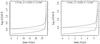 |
Fig. 1 Temporal evolution of the inner di and outer do boundaries of the HZ for host stars of M = 0.70 M⊙ (left panel) and M = 1.10 M⊙ (right panel) for Z = 0.005, Y = 0.2585 (i.e. ΔY/ ΔZ = 2), and To = 169 K. The HZ is the region between the two curves. The dashed lines mark the distance for which the HZ lasts longer. |
2.1. Stellar evolution models
The stellar models of this paper have been computed by means of the FRANEC (Degl’Innocenti et al. 2008) evolutionary code. We used
the most updated version of the code, with the same input physics and parameters as were
adopted to build the Pisa Stellar Evolution Data Base for low-mass stars1 (Dell’Omodarme et al.
2012; Dell’Omodarme & Valle 2013).
We followed the evolution from the pre-main sequence phase to the helium flash at the tip
of the red giant phase. Stellar tracks were computed in the mass range
[0.70−1.10] M⊙, with a step
of 0.05 M⊙, for metallicity Z in the range
[0.005−0.04], with a step of
0.005. We adopted the solar heavy elements mixture by Asplund et al. (2009). As usually done in literature, the value of the initial
helium abundance used as input parameter was obtained from the following linear relation:
 (4)with cosmological
4He abundance
value Yp = 0.2485, from WMAP
(Cyburt et al. 2004; Steigman 2006; Peimbert et al.
2007a,b), and assuming ΔY/ ΔZ =
2 (Pagel & Portinari
1998; Jimenez et al. 2003; Gennaro et al. 2010). To account for the current
uncertainty on ΔY/ ΔZ, models
with ΔY/
ΔZ = 1 and 3 were computed as well. We adopted our
solar calibrated value of the mixing length parameter, i.e. αml = 1.74.
Further details on the inputs adopted in the computations are available in Valle et al. (2009, 2013a,b).
(4)with cosmological
4He abundance
value Yp = 0.2485, from WMAP
(Cyburt et al. 2004; Steigman 2006; Peimbert et al.
2007a,b), and assuming ΔY/ ΔZ =
2 (Pagel & Portinari
1998; Jimenez et al. 2003; Gennaro et al. 2010). To account for the current
uncertainty on ΔY/ ΔZ, models
with ΔY/
ΔZ = 1 and 3 were computed as well. We adopted our
solar calibrated value of the mixing length parameter, i.e. αml = 1.74.
Further details on the inputs adopted in the computations are available in Valle et al. (2009, 2013a,b).
We computed 216 stellar evolutionary tracks specifically for the present work.
Relying on this fine grid of detailed stellar models, we make available an on-line tool2 that provides interpolated stellar tracks from the pre-main sequence to the red-giant branch tip for the required mass and chemical composition. The file provides as a function of time (in Gyr) the logarithm of stellar luminosity (in units of solar luminosity); the logarithm of the effective temperature (in K), the stellar mass (in units of solar mass); the initial helium content; the metallicity; the stellar radius (in units of solar radius); the logarithm of surface gravity (in cm s-2).
3. Results
In Fig. 1 we display the temporal evolution of the inner and outer boundaries – di and do – of the HZ, derived from Eq. (2) for stars with M = 0.70 and 1.10 M⊙ at Z = 0.005 and ΔY/ ΔZ = 2, assuming To = 169 K for the equilibrium temperature of the outer boundary. Figure 2 shows the same quantities but with respect to the logarithm of time, allowing the inspection of the pre-main sequence phase. The HZ is the region between the two boundaries. The figure shows that excluding the early pre-main sequence phase, the HZ moves progressively farther from the host star during its evolution as a consequence of the continuously growing luminosity. The time scale of this displacement depends on the evolutionary time scale of the host star. Thus, it is long during the main sequence phase and becomes much shorter after the central hydrogen depletion.
The duration of habitability at distance d is defined as the time interval for which the inequality di ≤ d ≤ do holds. If, for a given d, this inequality holds for multiple separated time intervals – as in the left panel of Fig. 2 – only the longest duration is considered. The dashed lines in the figures mark the distance dm for which the HZ has the maximum duration tm. Notice that dm corresponds to the value of do when the host star is in its ZAMS stage.
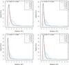 |
Fig. 3 Top row: duration of habitability (transit) as a function of the distance from the host star, for different masses M and chemical compositions of the host star for a fixed value of ΔY/ ΔZ = 2 and two metallicities Z = 0.005 and Z = 0.040. Bottom: same as the top row, but for a fixed metallicity Z = 0.040 and two values of ΔY/ ΔZ, namely 1 (left panel) and 3 (right panel). |
Figure 3 shows the duration of the habitability, also known as transit, as a function of the distance from the host star for different stellar masses and chemical compositions. The two panels of the top row adopt a fixed ΔY/ ΔZ = 2 but different metallicities, namely Z = 0.005 (left) and Z = 0.04 (right). The two panels of the bottom row have a fixed metallicity Z = 0.04 but different ΔY/ ΔZ values, namely 1 (left) and 3 (right). For a given chemical composition, the more massive the host star, the farther the HZ, the larger dm, and the shorter the transit duration tm. This is the expected consequence of the increasing brightness and decreasing lifetime of the host star as the mass increases. The plateau around the longest duration for masses higher than about 1.0 M⊙ is due to the drop in the luminosity of these stars after the central hydrogen depletion in the sub-giant branch (see e.g. the right panel of Fig. 1, around 5.2 Gyr). From the comparison of the two top panels it follows that a metallicity increase at fixed ΔY/ ΔZ leads to a decrease of dm and to an increase of the longest habitability duration tm. This behaviour can be easily understood by recalling that metal-rich stars evolve slower and fainter than metal-poor ones of the same mass. The comparison of the two bottom panels shows that a ΔY/ ΔZ increase at fixed metallicity Z leads to an increase of dm and a decrease of tm, that is, the opposite effect of increasing Z. Again, this is the consequence of the well-known dependence of stellar characteristics on the initial helium abundance: at a given mass and Z, the higher Y and the brighter and faster the evolution of a star. The steps that appear in the transit computed with high initial helium abundance for M = 1.1 M⊙ are due to the development of a convective core, which produces a step in the rate of the luminosity evolution with time. Figure 4 shows the same quantities, but for the logarithm of the transit time. The transformation allows a better display of the transit during the red-giant branch evolution of the host star.
The results presented here agree fairly well with those reported in Danchi & Lopez (2013). In the quoted paper, for an host star of 1.0 M⊙ with metallicity Z = 0.017 and Y = 0.26, the distance corresponding to the longest transit is around 1.7 AU, with a longest habitability duration slightly higher than 10 Gyr. In the present work, for a host star of 1.0 M⊙, metallicity Z = 0.015, and Y = 0.263 we found dm = 1.9 AU, and tm = 11.8 Gyr. Other comparisons are less meaningful since the initial helium content for different metallicities is chosen in a different way in the two works.
We focused our analysis on some features of the HZ; in addition to dm (in AU) and tm (in Gyr) defined above, we examined the width W (in AU) of the zone for which the habitability lasts tm/ 2, and the integral I (in AU Gyr) of the transit function for transits longer than 4 Gyr. These four quantities allow characterising the transit function in the most interesting region, where the transit time exceeds a few Gyr.
Figures 5 and 6 show the trend of the four chosen features with respect to the mass and metallicity of the host star. The distance dm corresponding to the longest HZ duration monotonically increases with the mass, while it decreases with Z toward a plateau for Z ≥ 0.03. The trend for W is the same as that for dm, while that for tm is reversed. For I, the effect of the metallicity is not monotonic: I reaches a maximum around Z = 0.03, with small variations in the Z range [0.02−0.04]. This trend results from the combination of an increase with Z of longest time of habitability tm, which is steeper for a metallicity below about Z = 0.02, with the trend of dm, which changes more smoothly with metallicity.
A high value of I is preferable in the observational target selection, since it is related to two desirable characteristics. The larger I, the larger either the extension of the 4 Gyr CHZ – implying higher chances that an exoplanet actually lies inside it – or the longer the habitability duration inside the CHZ – implying higher chances that an exoplanet in the 4 Gyr CHZ is indeed in a region that is continuously habitable for more than 4 Gyr. Since the curves in the different panels of Figs. 5 and 6 are not parallel, there is an effect due to the interaction between mass and metallicity, which means that the effect of changing the former quantity also depends on the value of the latter.
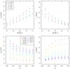 |
Fig. 5 Top row: the distance dm (in AU) for which the duration of the habitability is longest and the corresponding duration tm (in Gyr) as a function of the mass of the host star computed for different metallicities Z. Bottom row: dm (in AU) and tm (in Gyr) as a function of the metallicity of the star computed for different masses M. The value of initial helium abundance is derived assuming ΔY/ ΔZ = 2. |
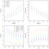 |
Fig. 6 As in Fig. 5, but for W, i.e. the width (in AU) of the zone for which the habitability lasts tm/ 2, and I, i.e. the integral (in AU Gyr) of the transit function for transits longer than 4 Gyr. |
The quantities discussed above are of relevant interest in the framework of the analysis of the impact of the stellar evolution on the HZ. However, to plan of a survey for life signature in exoplanet atmospheres, the most interesting feature is the CHZ boundaries position.
Figure 7 shows the position of the inner (Ri, left panel) and outer (Ro, right panel) boundaries of the 4 Gyr CHZ as a function of the host star mass for three ΔY/ ΔZ values, namely 1, 2, and 3. This allows exploring the effect of changing the initial helium abundance following Eq. (4). To improve the figure readability the abscissa of stars with high (low) helium-to-metal enrichment ratio is shifted by adding (subtracting) 0.005 M⊙. As expected, Ri and Ro increase with mass and decrease with metallicity. The temperature To of the outer boundary has no influence on the determination of the inner boundary. The spread of Ri and Ro with metallicity increases when mass and ΔY/ ΔZ increase. This suggests that interaction of metallicity, mass and helium content are important in determining the boundaries. The effect of a change of ΔY/ ΔZ for M = 1.1 M⊙ can be as large as 0.32 AU for Z = 0.04, while it decreases to a maximum of 0.12 AU for Z = 0.005. In the right panel of the figure we also show the effect of the change of To on the outer boundary. In this case, the effect of the change of the initial helium content is as large as 0.26 AU for Z = 0.04 and M = 1.1 M⊙ in the case of To = 169 K, and it decreases to a maximum of 0.19 AU for Z = 0.04 and To = 203 K. For the lowest analysed metallicity, Z = 0.005, these values drop to 0.025 AU and 0.015 AU.
The effect of varying the initial helium content is also displayed in Fig. 8, which shows the relative variation of the inner and outer boundaries of the CHZ for a change on the helium-to-metal enrichment from ΔY/ ΔZ = 3 to ΔY/ ΔZ = 1. For Ri (left panel) the relative variation ranges from about 5% for Z = 0.005 to about 30% for Z = 0.04, and it generally increases with the mass of the star. The decrease of variation that occurs for models of 1.1 M⊙ at high metallicities is due to the development of a convective core for the helium-rich models, which causes a step in the transit curve (see the bottom row in Fig. 3). For Ro (left panel in Fig. 8), assuming To = 169 K, the relative variation ranges from about 3% for Z = 0.005 to about 10% for Z = 0.04, and it generally mildly decreases with the mass of the star. As in the case discussed above, the exception are the models of 1.1 M⊙ at high metallicity.
The comparison of the result obtained in this work for a 1.0 M⊙ model with the corresponding one presented in Danchi & Lopez (2013) – who adopted a similar approach – requires some ad hoc calculations since in the quoted paper the boundaries of CHZ was computed for durations of 1 and 3 Gyr. The CHZ boundaries for an host star of 1.0 M⊙, Z = 0.017, and Y = 0.26 were reported to be [0.8−3.3] AU, and [0.9−2.8] AU for a duration of 1 and 3 Gyr, respectively. The corresponding values computed ad-hoc for the model of 1.0 M⊙, Z = 0.015, and Y = 0.263 are [0.84−3.56] AU and [0.90−2.94] AU, respectively.
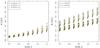 |
Fig. 7 Left: position (in AU) of the 4 Gyr CHZ inner boundary as a function of the host star mass for the labelled ΔY/ ΔZ values. For each set of mass and ΔY/ ΔZ, the metallicity Z runs from 0.04 at the upper point to 0.005 at the lower one. The initial helium content is obtained from Z and ΔY/ ΔZ as in Eq. (4). To show the effect of the initial helium content, the abscissa of models with high (low) ΔY/ ΔZ are shifted by adding (subtracting) 0.005 M⊙. Right: same as the left panel, but for the outer boundary. The circles correspond to the computations with To = 169 K, while the triangles correspond to those with To = 203 K. |
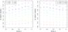 |
Fig. 8 Left: relative variation for a change from ΔY/ ΔZ = 3 to ΔY/ ΔZ = 1 of the 4 Gyr CHZ inner boundary as a function of the host star mass for the labelled Z values. Right: same as the left panel, but for the outer boundary. The adopted outer boundary temperature is To = 169 K. |
4. Analytical models
The dataset of computed stellar models allows a statistical analysis of the dependence of the previously discussed features on the host stellar characteristics. This analysis has three purposes. First, it allows distinguishing the contribution of the various input to the temporal variation of the HZ and the CHZ positions. Second, it provides an accurate and precise analytical model that can be safely used to evaluate the required characteristics without the need of time-consuming stellar model computations. As already discussed in Sect. 2, more than on actual estimates resulting from the models, we are interested in showing the degree of precision that can be reached – given a HZ defining scenario – by analytical relations. Third, these accurate models allow an uncertainty analysis to be performed (see Sect. 4.1) without the need to compute the huge number of detailed stellar models that would otherwise have been required.
The analysis was conducted by adapting linear models on the data, assuming dm, tm, W, Ri, and Ro as dependent variables and the mass of the host star M, the metallicity Z, and the initial helium abundance Y as independent variables (or covariates). The temperature of the outer boundary To is also inserted in the statistical models. Including this quantity in the analytical models allows the description of the HZ characteristics for a wide range of assumptions on To. This is especially useful since the determination of the outer boundary temperature strongly depends on the cloud coverage, which is not accurately described in the 1D climate models.
The building of the statistical models requires several checks. We started with simple
relations including linearly the covariates, but allowing for interaction between chemical
inputs (Z and
Y), the mass
of the star, and the boundary temperature. Then we checked whether the model was able to
describe all significant trends in the data without over-fitting them (see e.g. Faraway 2004). The first requirement was tackled by the
analysis of the standardised residuals, to check that the entire information of the data is
extracted by the model. The plots of the standardised residuals versus the covariates were
used to infer the need to include quadratic or cubic terms or high-order interactions. As a
result we obtained that although quadratic models are able to explain the bulk of data
variability, they are statistically unacceptable since clear trends remain in the residuals.
Cubic terms and more complex interactions are therefore needed in the models. The problem of
possible over-fitting required using the stepwise regression (Venables & Ripley 2002) technique, which allows one to evaluate
the performance of the multivariate model (balancing the goodness-of-fit and the number of
covariates in the model) and of the models nested in this one (i.e. models without some of
the covariates). To perform the stepwise model selection we employed the Bayesian
information criterion (BIC):  (5)which balances the
number of covariates p included in the model and its performance in the data
description, measured by the error deviance
(5)which balances the
number of covariates p included in the model and its performance in the data
description, measured by the error deviance  (n is the
number of points in the model). Among the models explored by the stepwise technique we
selected that with the lowest BIC value as the best one. The models were fitted to the data
with a least-squares method using the software R 3.0.2 (R
Development Core Team 2013).
(n is the
number of points in the model). Among the models explored by the stepwise technique we
selected that with the lowest BIC value as the best one. The models were fitted to the data
with a least-squares method using the software R 3.0.2 (R
Development Core Team 2013).
An interactive web code and a C program to obtain the HZ and CHZ characteristics described by the analytical models presented in this section are available on-line3. The web interface also computes an interpolated stellar track – from pre-main sequence to the helium flash at the red-giant branch tip – for the model of mass, metallicity, and initial helium content required by the user. The file provides as a function of time (in Gyr) the logarithm of stellar luminosity (in units of solar luminosity); the logarithm of the effective temperature (in K), the stellar mass (in units of solar mass); the initial helium content; the metallicity; the stellar radius (in units of solar radius); the logarithm of surface gravity (in cm s-2). The values can be useful for computing synthetic spectra of the incoming radiation to be coupled to climate models.
To concisely describe the analytical models, in this section we use the operator ∗, defined as A ∗ B ≡ A + B + A·B, and we excluded the regression coefficients in the models. The full forms of the models are reported in Appendix A.
The analytical model for the distance dm at which the HZ has the longest
duration is  (6)where Zl =
log Z, and K1 is a scaling factor that takes into
account different choices for the values of albedo A and To:
(6)where Zl =
log Z, and K1 is a scaling factor that takes into
account different choices for the values of albedo A and To:
 ,
T169 =
To/ (169K). The terms that
are selected in the stepwise procedure described above are reported in Table 1. The first two columns of the table report the
least-squares estimates of the regression coefficients and their errors; the third column
reports the t-statistic for the tests of the statistical significance
of the covariates; the fourth column reports the p-values of these tests. The left panel of Fig. 9 shows the relative error on the position of the maximum,
i.e.
,
T169 =
To/ (169K). The terms that
are selected in the stepwise procedure described above are reported in Table 1. The first two columns of the table report the
least-squares estimates of the regression coefficients and their errors; the third column
reports the t-statistic for the tests of the statistical significance
of the covariates; the fourth column reports the p-values of these tests. The left panel of Fig. 9 shows the relative error on the position of the maximum,
i.e.  where
where  is the position estimated from the linear model, as a function of log dm. The
relative errors are seldom greater – in modulus – than 0.4%, implying a good accuracy of the
estimates provided by Eq. (6).
is the position estimated from the linear model, as a function of log dm. The
relative errors are seldom greater – in modulus – than 0.4%, implying a good accuracy of the
estimates provided by Eq. (6).
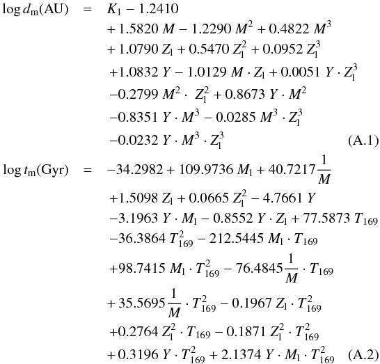
The analytical model for the longest duration tm (in Gyr) of the HZ is 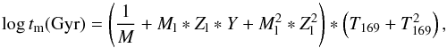 (7)where Ml =
log M/M⊙.
In this model the dependence on T169 must be explicitly included since
there is no simple geometrical scaling as in the case of dm. The terms
selected in the stepwise procedure described above are reported in Table 2. The central panel of Fig. 9 shows the relative error on tm as resulting from the estimates of Eq.
(7). In this case, the model relative
errors are greater than the ones for dm, but are seldom greater than 2% in
modulus.
(7)where Ml =
log M/M⊙.
In this model the dependence on T169 must be explicitly included since
there is no simple geometrical scaling as in the case of dm. The terms
selected in the stepwise procedure described above are reported in Table 2. The central panel of Fig. 9 shows the relative error on tm as resulting from the estimates of Eq.
(7). In this case, the model relative
errors are greater than the ones for dm, but are seldom greater than 2% in
modulus.
The analytical model for W (in AU) of the HZ is  (8)where the scaling
 accounts for possible different choices of the albedo A. The terms selected in the
stepwise procedure are reported in Table 3. The right
panel of Fig. 9 shows the relative error on
W as
resulting from the estimates of Eq. (8). The
dispersion of the relative errors is almost of the same magnitude of the one for
tm.
accounts for possible different choices of the albedo A. The terms selected in the
stepwise procedure are reported in Table 3. The right
panel of Fig. 9 shows the relative error on
W as
resulting from the estimates of Eq. (8). The
dispersion of the relative errors is almost of the same magnitude of the one for
tm.
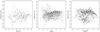 |
Fig. 9 Left: relative errors (positive values correspond to overestimated values) on the distance dm at which the HZ has the longest duration, as estimated from the model in Eq. (6). Middle: relative errors on the longest duration tm, as estimated from the model in Eq. (7). Right: relative errors on width at half maximum W, as estimated from the model in Eq. (8). |
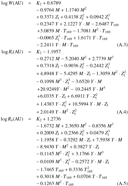
Regarding the 4 Gyr CHZ, the analytical model for the inner boundary Ri is
 (9)The terms that are selected
in the stepwise procedure are reported in Table 4.
The left panel of Fig. 10 shows the relative error in
Ri
as resulting from the estimates of Eq. (9).
The relative error is generally lower than 0.5%, so the model description of the CHZ inner
boundary trend is fairly accurate.
(9)The terms that are selected
in the stepwise procedure are reported in Table 4.
The left panel of Fig. 10 shows the relative error in
Ri
as resulting from the estimates of Eq. (9).
The relative error is generally lower than 0.5%, so the model description of the CHZ inner
boundary trend is fairly accurate.
For the outer boundary Ro, the dependence on the outer
temperature T169 is included in the model:  (10)The terms selected in
the stepwise procedure are reported in Table 5. The
relative error on Ro, as resulting from the estimates of Eq.
(9), is shown in the right panel of Fig.
10. The relative error is generally lower than 0.3%,
so the outer boundary is described with higher accuracy than the inner one.
(10)The terms selected in
the stepwise procedure are reported in Table 5. The
relative error on Ro, as resulting from the estimates of Eq.
(9), is shown in the right panel of Fig.
10. The relative error is generally lower than 0.3%,
so the outer boundary is described with higher accuracy than the inner one.
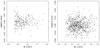 |
Fig. 10 Left: relative errors on the distance Ri of the inner boundary of the 4 Gyr CHZ, as estimated from the analytical model in Eq. (9). Right: as in the left panel, but for the CHZ outer boundary Ro, as estimated from the analytical model in Eq. (10). |
4.1. Sensitivity to the uncertainties in stellar mass and metallicity estimates
The statistical models described in the previous section allow determining the HZ and CHZ characteristics without the need to rely on time-consuming stellar evolution computations, after the mass and the metallicity of the host star are known. In the real world these quantities are subject to measurement or estimation errors, which propagate into the model output. Thus, it is important to estimate how the current uncertainties in the model input impact on the inferred CHZ boundaries. To our knowledge, this analysis is still lacking in the literature; this is the first attempt to quantitatively estimate the uncertainty propagation.
More in detail we evaluated, by means of Monte Carlo simulations, the relative variations on Ri and Ro induced by an uncertainty of 0.1 dex on log Z and of 0.05 M⊙ on the mass of the host star. These values are conservative estimates of the expected errors in [Fe/H] by spectroscopic measurements and of those in the stellar mass estimation by means of grid techniques in presence of asteroseimic constraints (see e.g. Quirion et al. 2010; Gai et al. 2011; Basu et al. 2012; Torres et al. 2012; Valle et al. 2014).
We define (Mi,Zi) as the vector composed by one of the 17 mass values in the range [0.7−1.1] M⊙ with a step of 0.025 M⊙ and one of the 15 metallicity values in the range [0.005−0.04] with a step of 0.0025. We adopted in these computations a value of ΔY/ ΔZ = 2. Let σ = (0.05,0.1) be the vector of the uncertainties in mass and log metallicity. We sampled 105 values of mass and metallicity assuming a multivariate normal distribution with vector of mean (Mi,log Zi) and diagonal covariance matrix Σ = diagσ2. For each of these combination we evaluated Ri and Ro from the statistical models described in Eqs. (9) and (10). Due to the asymmetry of the obtained distributions, as a dispersion measure we computed ΔRi and ΔRo as the differences between the 84th and the 16th quantile of the two distributions. The relative variation is obtained by the ratio of these values and that obtained for the reference point (Mi,Zi).
Figure 11 displays the contour plot of the relative variation on Ri (left) and Ro (right) in dependence on the mass and metallicity of the host star. The inner boundary of the CHZ is most sensitive to the uncertainty of the model input, with a relative variation ranging from about 27% to 37%, the higher values occurring at low metallicity. The relative variation of the outer boundary is about one half of that of the inner boundary and it increases at low mass.
To separate the contributions to the relative variation due to the uncertainties in mass and metallicity, we evaluated for each reference point described above ΔRi and ΔRo due to a variation of the mass Mi ± 0.05 M⊙ and of the metallicity log Zi ± 0.1 dex. Let ΔRi,M and ΔRo,M be the variation in the inner and outer boundary due to the mass uncertainty, and ΔRi,Z and ΔRo,Z the corresponding one due to the metallicity uncertainty. The left panel of Fig. 12 shows the contour plot of the ratio (ΔRi,M/ ΔRi,Z) with respect to the mass and metallicity of the host star. The right panel of the figure shows the corresponding quantities for the outer boundary. The contribution of the mass uncertainty is always greater than that due to the uncertainties in metallicity estimates and the difference increases towards low masses and low metallicities.
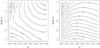 |
Fig. 11 Left: contour plot of the relative variation ΔR in Ri due to the simultaneous variation of the mass and the metallicity of the host star within their uncertainty ranges (see text for details). Right: as in the left panel for the outer radius Ro. We adopted ΔY/ ΔZ = 1. |
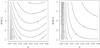 |
Fig. 12 Left: contour plot of the ratio (ΔRi,M/ ΔRi,Z), i.e. the ratio of the variation of the inner boundary Ri due to the change of the host star mass to the one due to metallicity change. Mass and metallicity are changed within their uncertainty ranges (see text for details). Right: as in the left panel, but for the outer radius Ro. We adopted ΔY/ ΔZ = 1. |
5. Excluding the constant albedo assumption
The results presented in the previous section mainly rely on the climatic computations presented in Kasting et al. (1993). These models have recently been revised by K13, who presented an updated and improved climate model obtaining new estimates for HZ. For our purposes the most relevant difference is that in computing the HZ boundaries we no longer assume a constant albedo at a given equilibrium temperature. The purpose of this section is to assess the effect of this modification on the discussed HZ characteristics.
To compute the incident flux the “BT Settl” grid of atmospheric models (Allard et al. 2007) has been adopted in K13. Solar metallicity was adopted in the computations (Kopparapu 2014, priv. comm.).
K13 reported a parametrisation of the Seff in dependence on the effective temperature of the star, for several explored HZ extensions. In the following we refer to their “moist greenhouse” for the inner boundary and “maximum greenhouse” for the outer one.
For inner and outer boundaries the critical effective flux is obtained by the relations
 (11)where T∗ =
Teff − 5780 K. The values of the
coefficients a,b,c,d are given in Table 3 of K13. The boundaries of
the HZ are then obtained from Eq. (1).
(11)where T∗ =
Teff − 5780 K. The values of the
coefficients a,b,c,d are given in Table 3 of K13. The boundaries of
the HZ are then obtained from Eq. (1).
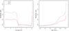 |
Fig. 13 Left: ratio of the inner and outer boundaries for the solar model obtained from the new climate models of Kopparapu et al. (2013) and the reference scenario. The temperature adopted for the outer boundary computation is To = 203 K. Right: detail of the red-giant branch evolutionary stage. |
With respect to our reference scenario, a systematic bias is expected on both the inner and the outer boundaries of the HZ since the critical effective stellar fluxes for the solar model of K13 are different from those adopted in Sect. 3. These biases can be computed – as resulting from Eq. (1) – from the square root of the ratio of the effective stellar fluxes of the two scenarios, and are about 11% and 7% on the inner and outer boundary. The changes of these biases with time will reveal the importance of taking into account the planetary albedo change during stellar evolution.
All these effects are shown in Fig. 13 for a model of 1.0 M⊙, Z = 0.015 (assuming ΔY/ ΔZ = 1)4. The figure shows the ratio of the inner and outer boundaries obtained from Eq. (11) and (1) with respect to those of our reference scenario, corrected for the multiplicative systematic biases due to the different solar critical fluxes adopted, as a function of the time. During the main sequence and sub-giant branch evolution the ratios between the HZ boundary estimates are close to 1.0 (the largest difference is smaller than 0.5%). As expected, the differences are larger during the pre-main sequence and the red-giant branch (RGB) phases, where the approximation of constant albedo is more problematic because of the large change in effective temperature with respect to the solar one. The difference in the computations for the inner and the outer boundary is about 5% and 12% in the pre-main sequence of the stellar evolution, and it can be as large as 25% for the outer boundary at the RGB tip. A systematic shift in MS is present for stars of different mass, because of the differences in their effective temperature. For a star of 0.7 M⊙ the typical biases in MS are about 4.5% and 10% at inner and outer boundary, while for a model of 1.1 M⊙ they are − 1.2% and − 2.5%.
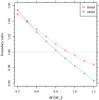 |
Fig. 14 Ratio of the inner and outer boundaries of the 4 Gyr CHZ obtained from the new climate models of Kopparapu et al. (2013) and the reference scenario. The temperature adopted for the outer boundary computation is To = 203 K. |
To evaluate the relevance of this effect, these values can be compared with those arising
from the current uncertainty in the stellar observables affecting the estimates of the
quantities in Eq. (1). In fact, these
uncertainties can lead to large variations on the actual HZ determination (see e.g. the
discussion in Kaltenegger & Sasselov 2011).
For the computation, we assumed 100 K as a conservative uncertainty in Teff (see e.g.
Gai et al. 2011; Basu et al. 2012; Valle et al. 2014).
Regarding the intrinsic luminosity, whenever no accurate distance are available (as for the
majority of the Kepler targets), an estimate of the uncertainty can be
obtained from the Stefan-Boltzmann relation  , where
R is the
stellar radius and σ is the Stefan-Boltzmann constant. In presence of
asteroseismic constraints a relative error on the stellar radius of about 2.5% can be
reached by means of grid-based techniques (Basu et al.
2012; Mathur et al. 2012; Valle et al. 2014). We adopted a 5% relative error in
radius as a more conservative estimate, accounting for the variability arising from
different estimation pipelines. By simple error propagation it is then possible to estimate
an uncertainty of about 12% on L for solar effective temperature. Then, the error
propagation in Eq. (1) shows that the
relative error on the derived boundary distances, due only to the current observational
uncertainty, is of about 6%. In summary, excluding the constant albedo has – on the HZ
characteristics evaluated on this paper – an influence that is lower than or equal to the
observational uncertainties, except for the outer boundary of our lowest mass model.
, where
R is the
stellar radius and σ is the Stefan-Boltzmann constant. In presence of
asteroseismic constraints a relative error on the stellar radius of about 2.5% can be
reached by means of grid-based techniques (Basu et al.
2012; Mathur et al. 2012; Valle et al. 2014). We adopted a 5% relative error in
radius as a more conservative estimate, accounting for the variability arising from
different estimation pipelines. By simple error propagation it is then possible to estimate
an uncertainty of about 12% on L for solar effective temperature. Then, the error
propagation in Eq. (1) shows that the
relative error on the derived boundary distances, due only to the current observational
uncertainty, is of about 6%. In summary, excluding the constant albedo has – on the HZ
characteristics evaluated on this paper – an influence that is lower than or equal to the
observational uncertainties, except for the outer boundary of our lowest mass model.
Moreover, the estimates of the HZ boundaries are affected by the uncertainties in the critical stellar fluxes resulting from different climate models. The observational uncertainty evaluated above is quite relevant as long as the HZ inner edge distance is evaluated, while it could be negligible for the outer edge. As an example, in the former case, for the solar model the estimate of the inner boundary of the HZ from 3D climate model of Leconte et al. (2013a) is 0.95 AU, while that from the 1D climate model presented in K13 is 0.99 AU, i.e. a relative variation of about 4%. In contrast, for the HZ outer boundary, the differences among the critical fluxes computed by climate models are still larger than the observational uncertainty (see e.g. the discussion in Selsis et al. 2007; Kaltenegger & Sasselov 2011).
The impact of excluding the constant albedo assumption on the HZ and CHZ characteristics discussed in Sect. 3 is expected to be of a few percent, since these characteristics are mainly based on the main-sequence stages of stellar evolution. To verify this point we evaluated the impact of the K13 climate model on the 4 Gyr CHZ boundaries for metallicity Z = 0.015 (with ΔY/ ΔZ = 1). The comparison of results for different Z are less meaningful since the correction of the effective flux does not take into account the metallicity of the host star. Although metallicity-related modifications to the spectrum of the incoming radiation in the climate model would introduce little modifications on the parametrisation presented in Eq. (11) (Kopparapu, 2014, priv. comm.), we avoided this possible source of bias and restricted ourself to solar metallicity.
Figure 14 shows the ratio of the inner and outer boundaries of the CHZ obtained by adopting the K13 parametrisation of the effective flux and those presented in the previous section. The inner and outer estimates of the reference scenario are corrected for the multiplicative biases discussed above, to account for the differences in the critical solar fluxes. For the model of 1.0 M⊙ the differences in the estimated boundaries are of about − 0.5% and − 2.0% for the inner and outer boundary. The maximum differences are about 5.0% and 5.5% for inner and outer boundary for the model of 0.70 M⊙. At 1.1 M⊙ the differences are about − 1.5% and − 3.5% for inner and outer boundary. The range of variation due to excluding the constant albedo hypothesis are thus much lower than the half-range of variation due to stellar mass and metallicity uncertainty presented in Sect. 4.1.
6. Conclusions and discussion
We studied the temporal evolution of the main quantities characterising the HZ of low-mass stars from pre-main sequence phase to the helium flash at the red-giant branch tip.
We computed a fine grid of detailed stellar models in the mass range [0.70−1.10] M⊙, for different metallicities Z (i.e. from 0.005 to 0.04), and different initial helium abundances Y (ΔY/ ΔZ = 1, 2, and 3).
To define habitability characteristics we focused our analysis on some features, such as the distance dm (in AU) for which the duration of habitability is longest, the corresponding duration tm (in Gyr), the width W (in AU) of the zone for which the habitability lasts tm/ 2, and the integral I (in AU Gyr) of the transit function for transits longer than 4 Gyr. We also evaluated the inner (Ri) and outer (Ro) boundaries of the 4 Gyr CHZ, which are useful for planning a survey for life signatures in exoplanet atmospheres.
The large set of computed stellar models allowed the fit of analytical linear models for dm, tm, W, Ri, and Ro. We found that the relative error of the analytical models on the estimated characteristics is of the order of a few percent or lower. Thus, these accurate analytical models allowed us to perform the first systematic study of the variability of the HZ boundaries position due to the uncertainty in the estimates of the host star mass and metallicity, without the need to compute a huge number of detailed, but time-consuming, stellar models.
A C program to compute the HZ and CHZ characteristics and an interactive web form are available on-line5. The web interface also allows interpolating stellar tracks for the required mass and chemical composition relying on our fine grid of stellar models. These tracks can be useful for computing synthetic spectra of the incoming radiation to be coupled to detailed climate models.
As expected and already shown by Danchi & Lopez (2013), the metallicity plays a relevant role in the HZ evolution: the duration of habitability at a given distance is longer for metal-rich stars than for metal-poor ones. The HZ and CHZ for high-metallicity stars are closer to the host star than those around low metallicity stars. For the first time, we also studied the effect of initial helium abundance; the increase of its value has an effect that is opposite to that of increasing metallicity.
The analytical models allowed us to evaluate the uncertainties on the derived boundaries of the CHZ due to the unavoidable errors on the mass and metallicity estimates of the host star. These values are in fact subject to observational or estimation uncertainties that propagate in the model output. Assuming an error of 0.05 M⊙ and 0.1 dex in the mass and log metallicity, we found that the relative variation of the inner boundary position ranges from about 27% to 37%, while that for the outer boundary is about one half of these values.
The initial helium content of the host star was found to affect the determination of the 4 Gyr CHZ boundaries in a non-negligible way, mainly the inner one. The helium variation considered in this paper, caused by varying ΔY/ ΔZ from 3 to 1, led to a relative variation of the position of Ri between about 5% for Z = 0.005 to about 30% for Z = 0.04. The relative variation of the outer boundary Ro is less important and is generally lower than 10%.
The results presented in this paper are the first study of the variability of the CHZ boundary position due to the uncertainty on the host star characteristics. This kind of variability is substantial and is of the same order or greater than the systematic uncertainty due to several other factors reported in recent literature, such as the use of different stellar evolution computations that adopt slightly different input physics, the refinement of climatic models, or the adoption of an integrated approach in the definition of the HZ.
The first of these effects was evaluated by a direct comparison of the results presented here with the only overlapping one obtained with a different stellar evolution code by Danchi & Lopez (2013). The comparison showed a difference in the CHZ boundary of less than 5%, a value higher than the random component due to linear modelling of Sect. 4, but much lower than the variability due to the uncertainties in the estimates of the mass and chemical composition of the host star.
The impact of different climate models on the HZ calculations is more difficult to assess since there are many parameters involved. However, some conclusions can be stated. The modifications to the climatic models of Kasting et al. (1993) presented by K13 and excluding the constant albedo assumption was evaluated by computing, for solar metallicity, the boundaries of the 4 Gyr CHZ adopting the estimates provided in K13. With respect to the results obtained with our reference scenario we found a maximum variation of about 4% at 0.7 M⊙ and − 3% at 1.1 M⊙. These uncertainties are much lower than those arising from the uncertainty in the estimates of stellar mass and metallicity. Moreover, K13 reported a comparison of their estimates with those by Selsis et al. (2007), who adopted another different approach to the boundary correction. The differences are lower than 6% for the inner boundary and even lower for the outer one.
The quantification of the internal uncertainty due only to stellar evolution was facilitated by the fact that the stellar models are based on a sound theory, with a relatively small set of input and parameters and that the results can be verified by comparison with large data sets. This is not the case for climatic or geophysics models of planets different from Earth, since these models depend on planetary parameters that are impossible to estimate before a planet has actually been discovered and characterised (see e.g. the extensive discussion in Selsis et al. 2007). Several efforts have been made to shed light on the impact of some potentially important effects due to planetary characteristics, such as the planetary mass (Kopparapu et al. 2014), its rotation speed (Yang et al. 2014), its tidal obliquity evolution, that is, the change of the angle between the planet rotational axis and the orbital plane normal (Heller et al. 2011). The impact of these planetary characteristics can be very strong: recent computations by means of a three-dimensional general circulation model by Yang et al. (2014) have shown that slowly rotating planets can maintain an Earth-like climate at nearly twice the stellar flux as rapidly rotating ones. These planet-specific parameters can be correctly taken into account only after a planet characterisation. More investigations that focus on the quantification of the internal uncertainty of these approaches are needed to assess the relative importance of the many source of uncertainty that concur in the HZ definition.
The main interest in defining the HZ is the hope of identifying an actually inhabited world. The key concept in this research area is to find a terrestrial exoplanet atmosphere severely out of thermochemical redox equilibrium (see e.g. Lovelock 1965; Seager 2013; Seager et al. 2013), assuming that life fundamental chemical reactions release biosignature gases – such as oxygen or ozone – as metabolic process by-products. The results presented in this work, suggesting good host star targets for the observational follow-up, can be useful for the planning of life-signature detection in exoplanet atmospheres.
The different established exoplanet atmosphere observational methods have different requirements in terms of location of the planetary target. Direct imaging of an exoplanet and its atmospheric characterisation impose severe requirements in terms of spatial resolution and contrast (see e.g. Seager & Deming 2010, for a review), and it is currently limited to bright and massive planets orbiting far from the host star.
A second way to study an exoplanet atmosphere composition is exploitable for transiting exoplanets, that is, exoplanets that cross the line of sight from Earth to the host star (see e.g. Seager & Deming 2010, and references therein). This allows characterising the flux spectrum of the planet. The likelihood of a transit configuration is higher for planets at a short distance from their host star. In the light of the results presented here, this is a favourable condition since the highest chances to find a planet in the 4 Gyr CHZ were found for low-mass, near-solar metallicity stars. In these cases the CHZ is close to the host star.
This set is the closest to our own standard solar model (Z = 0.0137, Y = 0.253) in the available grid of stellar models.
Acknowledgments
We are grateful to our anonymous referees for many stimulating suggestions and comments that were a great help to us in clarifying and improving the paper. We warmly thanks Ravi Kumar Kopparapu for his exhaustive answer to our request for information. We thank Paolo Paolicchi for carefully reading the paper and for useful comments. This work has been supported by PRIN-MIUR 2010-2011 (Chemical and dynamical evolution of the Milky Way and Local Group galaxies, PI F. Matteucci), PRIN-INAF 2011 (Tracing the formation and evolution of the Galactic Halo with VST, PI M. Marconi), and PRIN-INAF 2011 (The M4 Core Project with Hubble Space Telescope, PI L. Bedin).
References
- Allard, F., Allard, N. F., Homeier, D., et al. 2007, A&A, 474, L21 [NASA ADS] [CrossRef] [EDP Sciences] [Google Scholar]
- Anglada-Escudé, G., Arriagada, P., Vogt, S. S., et al. 2012, ApJ, 751, L16 [NASA ADS] [CrossRef] [Google Scholar]
- Asplund, M., Grevesse, N., Sauval, A. J., & Scott, P. 2009, ARA&A, 47, 481 [NASA ADS] [CrossRef] [Google Scholar]
- Barclay, T., Burke, C. J., Howell, S. B., et al. 2013, ApJ, 768, 101 [NASA ADS] [CrossRef] [Google Scholar]
- Basu, S., Verner, G. A., Chaplin, W. J., & Elsworth, Y. 2012, ApJ, 746, 76 [NASA ADS] [CrossRef] [Google Scholar]
- Batalha, N. M., Rowe, J. F., Bryson, S. T., et al. 2013, ApJS, 204, 24 [NASA ADS] [CrossRef] [Google Scholar]
- Batista, V., Beaulieu, J.-P., Gould, A., et al. 2014, ApJ, 780, 54 [NASA ADS] [CrossRef] [Google Scholar]
- Borucki, W. J., Koch, D. G., Basri, G., et al. 2011, ApJ, 736, 19 [NASA ADS] [CrossRef] [Google Scholar]
- Borucki, W. J., Koch, D. G., Batalha, N., et al. 2012, ApJ, 745, 120 [NASA ADS] [CrossRef] [Google Scholar]
- Buccino, A. P., Lemarchand, G. A., & Mauas, P. J. D. 2006, Icarus, 183, 491 [NASA ADS] [CrossRef] [Google Scholar]
- Cantrell, J. R., Henry, T. J., & White, R. J. 2013, AJ, 146, 99 [NASA ADS] [CrossRef] [Google Scholar]
- Cyburt, R. H., Fields, B. D., & Olive, K. A. 2004, Phys. Rev. D, 69, 123519 [NASA ADS] [CrossRef] [Google Scholar]
- Danchi, W. C., & Lopez, B. 2013, ApJ, 769, 27 [NASA ADS] [CrossRef] [Google Scholar]
- de Pater, I., & Lissauer, J. J. 2001, Planetary Sciences (Cambridge University Press) [Google Scholar]
- Degl’Innocenti, S., Pra da Moroni, P. G., Marconi, M., & Ruoppo, A. 2008, Ap&SS, 316, 25 [NASA ADS] [CrossRef] [Google Scholar]
- Dell’Omodarme, M., & Valle, G. 2013, The R Journal, 5, 108 [Google Scholar]
- Dell’Omodarme, M., Valle, G., Degl’Innocenti, S., & Prada Moroni, P. G. 2012, A&A, 540, A26 [NASA ADS] [CrossRef] [EDP Sciences] [Google Scholar]
- Faraway, J. J. 2004, Linear Models with R (Chapman & Hall/CRC) [Google Scholar]
- Forget, F. 1998, Earth Moon and Planets, 81, 59 [NASA ADS] [CrossRef] [Google Scholar]
- Forget, F., & Pierrehumbert, R. T. 1997, Science, 278, 1273 [NASA ADS] [CrossRef] [PubMed] [Google Scholar]
- Gai, N., Basu, S., Chaplin, W. J., & Elsworth, Y. 2011, ApJ, 730, 63 [NASA ADS] [CrossRef] [Google Scholar]
- Gennaro, M., Prada Moroni, P. G., & Degl’Innocenti, S. 2010, A&A, 518, A13 [NASA ADS] [CrossRef] [EDP Sciences] [Google Scholar]
- Hart, M. H. 1978, Icarus, 33, 23 [NASA ADS] [CrossRef] [Google Scholar]
- Heller, R., Leconte, J., & Barnes, R. 2011, A&A, 528, A27 [NASA ADS] [CrossRef] [EDP Sciences] [Google Scholar]
- Jimenez, R., Flynn, C., MacDonald, J., & Gibson, B. K. 2003, Science, 299, 1552 [NASA ADS] [CrossRef] [PubMed] [Google Scholar]
- Kaltenegger, L., & Sasselov, D. 2011, ApJ, 736, L25 [NASA ADS] [CrossRef] [Google Scholar]
- Kasting, J. F., Whitmire, D. P., & Reynolds, R. T. 1993, Icarus, 101, 108 [NASA ADS] [CrossRef] [PubMed] [Google Scholar]
- Kopparapu, R. K., Ramirez, R., Kasting, J. F., et al. 2013, ApJ, 765, 131 (K13) [NASA ADS] [CrossRef] [Google Scholar]
- Kopparapu, R. K., Ramirez, R. M., SchottelKotte, J., et al. 2014, ApJ, 787, L29 [NASA ADS] [CrossRef] [Google Scholar]
- Leconte, J., Forget, F., Charnay, B., Wordsworth, R., & Pottier, A. 2013a, Nature, 504, 268 [NASA ADS] [CrossRef] [Google Scholar]
- Leconte, J., Forget, F., Charnay, B., et al. 2013b, A&A, 554, A69 [NASA ADS] [CrossRef] [EDP Sciences] [Google Scholar]
- Lopez, B., Schneider, J., & Danchi, W. C. 2005, ApJ, 627, 974 [NASA ADS] [CrossRef] [Google Scholar]
- Lovelock, J. E. 1965, Nature, 207, 568 [NASA ADS] [CrossRef] [PubMed] [Google Scholar]
- Mathur, S., Metcalfe, T. S., Woitaszek, M., et al. 2012, ApJ, 749, 152 [NASA ADS] [CrossRef] [Google Scholar]
- Mischna, M. A., Kasting, J. F., Pavlov, A., & Freedman, R. 2000, Icarus, 145, 546 [NASA ADS] [CrossRef] [PubMed] [Google Scholar]
- Pagel, B. E. J., & Portinari, L. 1998, MNRAS, 298, 747 [NASA ADS] [CrossRef] [Google Scholar]
- Peimbert, M., Luridiana, V., & Peimbert, A. 2007a, ApJ, 666, 636 [NASA ADS] [CrossRef] [Google Scholar]
- Peimbert, M., Luridiana, V., Peimbert, A., & Carigi, L. 2007b, in From Stars to Galaxies: Building the Pieces to Build Up the Universe, eds. A. Vallenari, R. Tantalo, L. Portinari, & A. Moretti, ASP Conf. Ser., 374, 81 [Google Scholar]
- Pepe, F., Lovis, C., Ségransan, D., et al. 2011, A&A, 534, A58 [NASA ADS] [CrossRef] [EDP Sciences] [Google Scholar]
- Pierrehumbert, R., & Gaidos, E. 2011, ApJ, 734, L13 [NASA ADS] [CrossRef] [Google Scholar]
- Quirion, P.-O., Christensen-Dalsgaard, J., & Arentoft, T. 2010, ApJ, 725, 2176 [NASA ADS] [CrossRef] [Google Scholar]
- R Development Core Team. 2013, R: A Language and Environment for Statistical Computing, R Foundation for Statistical Computing, Vienna, Austria [Google Scholar]
- Schopf, J. W. 1993, Science, 260, 640 [NASA ADS] [CrossRef] [PubMed] [Google Scholar]
- Seager, S. 2013, Science, 340, 577 [NASA ADS] [CrossRef] [Google Scholar]
- Seager, S., & Deming, D. 2010, ARA&A, 48, 631 [NASA ADS] [CrossRef] [Google Scholar]
- Seager, S., Bains, W., & Hu, R. 2013, ApJ, 775, 104 [NASA ADS] [CrossRef] [Google Scholar]
- Selsis, F., Kasting, J. F., Levrard, B., et al. 2007, A&A, 476, 1373 [NASA ADS] [CrossRef] [EDP Sciences] [Google Scholar]
- Steigman, G. 2006, Int. J. Mod. Phys. E, 15, 1 [Google Scholar]
- Stevenson, D. J. 1999, Nature, 400, 32 [NASA ADS] [CrossRef] [Google Scholar]
- Torres, G., Fischer, D. A., Sozzetti, A., et al. 2012, ApJ, 757, 161 [NASA ADS] [CrossRef] [Google Scholar]
- Tuomi, M., Anglada-Escudé, G., Gerlach, E., et al. 2013, A&A, 549, A48 [NASA ADS] [CrossRef] [EDP Sciences] [Google Scholar]
- Turnbull, M. C., & Tarter, J. C. 2003, ApJS, 149, 423 [NASA ADS] [CrossRef] [Google Scholar]
- Udry, S., Bonfils, X., Delfosse, X., et al. 2007, A&A, 469, L43 [NASA ADS] [CrossRef] [EDP Sciences] [Google Scholar]
- Underwood, D. R., Jones, B. W., & Sleep, P. N. 2003, Int. J. Astrobiol., 2, 289 [Google Scholar]
- Valle, G., Marconi, M., Degl’Innocenti, S., & Pra da Moroni, P. G. 2009, A&A, 507, 1541 [NASA ADS] [CrossRef] [EDP Sciences] [Google Scholar]
- Valle, G., Dell’Omodarme, M., Prada Moroni, P. G., & Degl’Innocenti, S. 2013a, A&A, 549, A50 [NASA ADS] [CrossRef] [EDP Sciences] [Google Scholar]
- Valle, G., Dell’Omodarme, M., Prada Moroni, P. G., & Degl’Innocenti, S. 2013b, A&A, 554, A68 [NASA ADS] [CrossRef] [EDP Sciences] [Google Scholar]
- Valle, G., Dell’Omodarme, M., Prada Moroni, P. G., & Degl’Innocenti, S. 2014, A&A, 561, A125 [NASA ADS] [CrossRef] [EDP Sciences] [Google Scholar]
- Venables, W., & Ripley, B. 2002, Modern applied statistics with S, Statistics and computing (Springer) [Google Scholar]
- von Bloh, W., Cuntz, M., Schröder, K.-P., Bounama, C., & Franck, S. 2009, Astrobiology, 9, 593 [NASA ADS] [CrossRef] [PubMed] [Google Scholar]
- Wordsworth, R. D., Forget, F., Selsis, F., et al. 2011, ApJ, 733, L48 [NASA ADS] [CrossRef] [Google Scholar]
- Yang, J., Boué, G., Fabrycky, D. C., & Abbot, D. S. 2014, ApJ, 787, L2 [NASA ADS] [CrossRef] [Google Scholar]
Appendix A: Detailed analytical models
For convenience, we report here the full form of the analytical models described in Sect.
4. As in the main text we define Zl =
log Z, Ml = log M,
 ,
T169 =
To/ (169K),
.
,
T169 =
To/ (169K),
.
All Tables
All Figures
|
Fig. 1 Temporal evolution of the inner di and outer do boundaries of the HZ for host stars of M = 0.70 M⊙ (left panel) and M = 1.10 M⊙ (right panel) for Z = 0.005, Y = 0.2585 (i.e. ΔY/ ΔZ = 2), and To = 169 K. The HZ is the region between the two curves. The dashed lines mark the distance for which the HZ lasts longer. |
| In the text | |
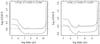 |
Fig. 2 As in Fig. 1, but for the logarithm of the time. |
| In the text | |
|
Fig. 3 Top row: duration of habitability (transit) as a function of the distance from the host star, for different masses M and chemical compositions of the host star for a fixed value of ΔY/ ΔZ = 2 and two metallicities Z = 0.005 and Z = 0.040. Bottom: same as the top row, but for a fixed metallicity Z = 0.040 and two values of ΔY/ ΔZ, namely 1 (left panel) and 3 (right panel). |
| In the text | |
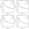 |
Fig. 4 As in Fig. 3, but for the logarithm of the transit time. |
| In the text | |
|
Fig. 5 Top row: the distance dm (in AU) for which the duration of the habitability is longest and the corresponding duration tm (in Gyr) as a function of the mass of the host star computed for different metallicities Z. Bottom row: dm (in AU) and tm (in Gyr) as a function of the metallicity of the star computed for different masses M. The value of initial helium abundance is derived assuming ΔY/ ΔZ = 2. |
| In the text | |
|
Fig. 6 As in Fig. 5, but for W, i.e. the width (in AU) of the zone for which the habitability lasts tm/ 2, and I, i.e. the integral (in AU Gyr) of the transit function for transits longer than 4 Gyr. |
| In the text | |
|
Fig. 7 Left: position (in AU) of the 4 Gyr CHZ inner boundary as a function of the host star mass for the labelled ΔY/ ΔZ values. For each set of mass and ΔY/ ΔZ, the metallicity Z runs from 0.04 at the upper point to 0.005 at the lower one. The initial helium content is obtained from Z and ΔY/ ΔZ as in Eq. (4). To show the effect of the initial helium content, the abscissa of models with high (low) ΔY/ ΔZ are shifted by adding (subtracting) 0.005 M⊙. Right: same as the left panel, but for the outer boundary. The circles correspond to the computations with To = 169 K, while the triangles correspond to those with To = 203 K. |
| In the text | |
|
Fig. 8 Left: relative variation for a change from ΔY/ ΔZ = 3 to ΔY/ ΔZ = 1 of the 4 Gyr CHZ inner boundary as a function of the host star mass for the labelled Z values. Right: same as the left panel, but for the outer boundary. The adopted outer boundary temperature is To = 169 K. |
| In the text | |
|
Fig. 9 Left: relative errors (positive values correspond to overestimated values) on the distance dm at which the HZ has the longest duration, as estimated from the model in Eq. (6). Middle: relative errors on the longest duration tm, as estimated from the model in Eq. (7). Right: relative errors on width at half maximum W, as estimated from the model in Eq. (8). |
| In the text | |
|
Fig. 10 Left: relative errors on the distance Ri of the inner boundary of the 4 Gyr CHZ, as estimated from the analytical model in Eq. (9). Right: as in the left panel, but for the CHZ outer boundary Ro, as estimated from the analytical model in Eq. (10). |
| In the text | |
|
Fig. 11 Left: contour plot of the relative variation ΔR in Ri due to the simultaneous variation of the mass and the metallicity of the host star within their uncertainty ranges (see text for details). Right: as in the left panel for the outer radius Ro. We adopted ΔY/ ΔZ = 1. |
| In the text | |
|
Fig. 12 Left: contour plot of the ratio (ΔRi,M/ ΔRi,Z), i.e. the ratio of the variation of the inner boundary Ri due to the change of the host star mass to the one due to metallicity change. Mass and metallicity are changed within their uncertainty ranges (see text for details). Right: as in the left panel, but for the outer radius Ro. We adopted ΔY/ ΔZ = 1. |
| In the text | |
|
Fig. 13 Left: ratio of the inner and outer boundaries for the solar model obtained from the new climate models of Kopparapu et al. (2013) and the reference scenario. The temperature adopted for the outer boundary computation is To = 203 K. Right: detail of the red-giant branch evolutionary stage. |
| In the text | |
|
Fig. 14 Ratio of the inner and outer boundaries of the 4 Gyr CHZ obtained from the new climate models of Kopparapu et al. (2013) and the reference scenario. The temperature adopted for the outer boundary computation is To = 203 K. |
| In the text | |
Current usage metrics show cumulative count of Article Views (full-text article views including HTML views, PDF and ePub downloads, according to the available data) and Abstracts Views on Vision4Press platform.
Data correspond to usage on the plateform after 2015. The current usage metrics is available 48-96 hours after online publication and is updated daily on week days.
Initial download of the metrics may take a while.