| Issue |
A&A
Volume 567, July 2014
|
|
|---|---|---|
| Article Number | A90 | |
| Number of page(s) | 8 | |
| Section | The Sun | |
| DOI | https://doi.org/10.1051/0004-6361/201323319 | |
| Published online | 17 July 2014 | |
Reversals of the solar magnetic dipole in the light of observational data and simple dynamo models
1
Institute of Solar-Terrestrial Physics RAS,
664033
Irkutsk,
Russia
e-mail:
This email address is being protected from spambots. You need JavaScript enabled to view it.
2
School of Mathematics, University of Manchester,
Oxford Road,
Manchester
M13 9PL,
UK
3
Department of Physics, Moscow University,
119992
Moscow,
Russia
4
W.W. Hansen Experimental Physics Laboratory, Stanford University,
Stanford
CA
94305,
USA
Received:
22
December
2013
Accepted:
18
June
2014
Abstract
Context. Observations show that the photospheric solar magnetic dipole usually does not vanish during the reversal of the solar magnetic field, which occurs in each solar cycle. In contrast, mean-field solar dynamo models predict that the dipole field does become zero. In a recent paper it was suggested that this contradiction could be explained as a large-scale manifestation of small-scale magnetic fluctuations of the surface poloidal field.
Aims. Our aim is to confront this interpretation with the available observational data.
Methods. Here we compare this interpretation with Wilcox Solar Observatory (WSO) photospheric magnetic field data in order to determine the amplitude of magnetic fluctuations required to explain the phenomenon and to compare the results with predictions from a simple dynamo model which takes these fluctuations into account.
Results. We demonstrate that the WSO data concerning the magnetic dipole reversals are very similar to the predictions from our very simple solar dynamo model, which includes both mean magnetic field and fluctuations. The ratio between the rms value of the magnetic fluctuations and the mean field is estimated to be about 2, in reasonable agreement with estimates from sunspot data. The reversal epoch, during which the fluctuating contribution to the dipole is larger than that from the mean field, is about 4 months. The memory time of the fluctuations is about 2 months. Observations demonstrate that the rms of the magnetic fluctuations is strongly modulated by the phase of the solar cycle. This gives additional support to the concept that the solar magnetic field is generated by a single dynamo mechanism rather than also by independent small-scale dynamo action. A suggestion of a weak nonaxisymmetric magnetic field of a fluctuating nature arises from the analysis, with a lifetime of about 1 year.
Conclusions. The behaviour of the magnetic dipole during the reversal epoch gives valuable information about details of solar dynamo action.
Key words: Sun: magnetic fields / Sun: activity / magnetic fields
© ESO, 2014
1. Introduction
Our research presented in this paper starts from the following quite simple statements. The photospheric solar magnetic dipole reverses its orientation every 11 years, in the course of the solar activity cycle. It is believed that the solar cycle is driven by a dynamo mechanism operating deep in the convection zone. The evolution of the solar dipole is synchronized with sunspot activity. Details of this synchronization may depend on the underlying dynamo mechanism (Pipin & Kosovichev 2013). Figure 1 shows reversals of the dipolar component of the large-scale magnetic field of the Sun.
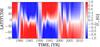 |
Fig. 1 Evolution of the dipole component of the radial magnetic field as obtained from measurements at the WSO from 1976 to 2013. |
The Sun is basically axisymmetric so a natural expectation is that the solar magnetic field is also approximately axisymmetric. Correspondingly, a standard mean-field description of the solar dynamo assumes axial symmetry and that the solar dipole vanishes at the instant of reversal. In contrast, observational data (Livshits & Obridko 2006; DeRosa et al. 2012) show that the solar magnetic dipole rotates from pole to pole during the course of a reversal, even becoming orthogonal to the rotation axis at some instant, this corresponding obviously to the vanishing of the polar dipole. At such a time the total magnetic field is strongly nonaxisymmetric.
Moss et al. (2013) suggested that this apparent contradiction is explicable as a manifestation of contributions from fluctuations of the surface magnetic field (specifically its poloidal component) near the moment of reversal. The aim of this paper is to develop and present a quantitative model that allows direct comparison of the interpretation of Moss et al. (2013) with observations. Using a simple simulation of this process, we produce models in which the trajectory of the dipole axis on the surface mimics well the observed behaviour. Other properties of the model also resemble those observed.
In this paper, we concentrate on the fact (known for some time from solar activity studies, but little exploited) that the large-scale magnetic field becomes substantially nonaxisymmetric during a reversal. Quantifying this nonaxisymmetry in terms offluctuations of the surface solar magnetic field, we suggest that something can be learned about the relative contributions of mean-field and small-scale dynamos to the solar magnetic field (Sect. 6). We note that the relationship between dipolar and quadrupolar modes in solar dynamo action was addressed by DeRosa et al. (2012) and we do not discuss it here. The manifestation of a substantial nonaxisymmetric component of the solar dipolar magnetic field is interpreted in the framework of mean-field dynamo theory.
One further point is that the apparent discrepancy between dynamo theory and the observations applies explicitly (in the form discussed above) only to mean-field dynamos. Of course, the solar magnetic field obtained from direct numerical simulations (DNS) is not strictly axisymmetric – even for hydrodynamics which is axisymmetric on average. In principle, one might prefer to use DNS and thus avoid any mean-field interpretation with its associated uncertainties, rather than involving magnetic fluctuations in the mean-field description. However, at the moment DNS models are expensive in terms of computing resources required. A hint that the sort of behaviour studied here may not be incompatible with DNS is given by Brown et al. (2011), where one model appears to show a latitudinal migration of the dipolar component. We believe that a mean-field formulation of dynamo theory is a fruitful way to obtain a qualitative understanding of the solar cycle, and to compare it with observations. Thus the formulation of an adequate description of the mean-field behaviour of the solar cycle is a desirable undertaking.
One outcome of the investigation presented here is the recognition that the observational analysis isolates some features of the solar dynamo that appear instructive and informative in various other contexts related to solar dynamos. We discuss such byproducts at the end of the paper (Sect. 6).
2. Methodology
Our tactic in comparing theory and observations is as follows. First we must understand the capability of a mean-field dynamo model in explaining the phenomenon under discussion. A reasonable approach is to take the simplest dynamo model, compare it with observations and then add more and more realistic details until the desired agreement is achieved. We start with the illustrative Parker (1955) dynamo model and find that it is adequate to provide the mean-field component of the theoretical modelling. This makes using a detailed mean-field model unnecessary at this stage. Of course, we recognize the purely illustrative nature of this toy model (for example, the incorrect phase relation between toroidal and poloidal magnetic fields); however such issues are not relevant for the point being discussed. Note that the primitive nature of this mean-field model allows us to introduce a parameter which quantifies the link between toroidal and poloidal magnetic field and so avoid any specific connection with the α-effect introduced by Steenbeck, Krause and Rädler (see Krause & Rädler 1980). Thus the results should also be applicable to flux-transport models (e.g. Choudhuri 2008).
Standard mean-field dynamo models do not contain explicit magnetic fluctuations and we have to include them somehow. This can be done in various forms and again we do it in the simplest way, i.e. by adding magnetic fluctuations “by hand” using a random number generator, as described in Sect. 4. This is found to be sufficient to reproduce the observational phenomenology. The reversal phenomenon is quite robust and does not depend on details of the model. We see below that the magnetic fluctuation properties from our analysis are meaningful for understanding the surface manifestations of solar dynamo action. Thus there is no motivation for considering more realistic dynamo models. Of course the true solar dynamo is much more complicated than the toy model we use to mimic the observations.
Various approaches have been discussed for determining the position of the solar magnetic pole, see, for example, Noonoj & Kuklin (1988) and de Patoul et al. (2013). A delicate feature of our analysis is the fact that the observational data exploited are observations of the magnetic field at the solar surface. Such a field is mainly contributed by the magnetic fields that originate in solar active regions, which in turn are mainly determined by the toroidal magnetic field within the Sun. On the other hand, we are interested in the solar dipole magnetic moment and the toroidal field gives no contribution to this quantity. Of course, the fact that only a tiny part of the surface magnetic field determines the quantity being discussed requires some care in using the data. We note however that the situation is recognized by solar observers who have verified the reliability of the result with great care.
3. Observational data
In the paper we analyze the components of the global magnetic field deduced from the daily magnetograph observations that have been made at the Wilcox Solar Observatory (WSO) at Stanford since May 1976. The solar magnetograph measures the line-of-sight component of the photospheric magnetic field with three arc min resolution (see details in Scherrer et al. 1977 and Duvall et al. 1977). This homogeneous data set provides information about the evolution of the photospheric magnetic field through the past three Solar Cycles, 21, 22 and 23. The daily magnetograms were interpolated on to the Carrington grid and assembled into synoptic charts which were further used to determine the coefficients of the spherical harmonics of the potential magnetic field outside of the Sun. The procedure is described in detail by Hoeksema & Scherrer (1996). Below, we discuss some particular points which are essential for the current study.
We consider the spherical harmonic decomposition of a scalar potential
![Mathematical equation: \begin{eqnarray} \psi=R\sum_{n=1}^{\infty}\sum_{m=0}^{n}\left(\frac{R}{r}\right)^{n+1}[g_{n}^{(m)}\cos\left(m\phi\right) +h_{n}^{(m)}\sin\left(m\phi\right)]P_{n}^{m}\left(\theta\right). \end{eqnarray}](/articles/aa/full_html/2014/07/aa23319-13/aa23319-13-eq2.png) (1)The
potential magnetic field above the solar surface can be represented as a gradient of a
scalar potential, B
= −∇ψ. The data reduction uses the calculations of the
radial harmonic coefficients of the photospheric magnetic field described by Zhao & Hoeksema (1993), see also Hoeksema & Scherrer (1996). Note, that the
fitting procedure is made using a radial magnetic field as a boundary condition (see Zhao & Hoeksema 1993). Coefficients of the
spherical harmonics are computed for each 10 degrees of Carrington rotation. In our analysis
we use the components of the axial and equatorial dipoles provided by the first three
coefficients of the potential field extrapolation of the photospheric magnetic field,
namely,
(1)The
potential magnetic field above the solar surface can be represented as a gradient of a
scalar potential, B
= −∇ψ. The data reduction uses the calculations of the
radial harmonic coefficients of the photospheric magnetic field described by Zhao & Hoeksema (1993), see also Hoeksema & Scherrer (1996). Note, that the
fitting procedure is made using a radial magnetic field as a boundary condition (see Zhao & Hoeksema 1993). Coefficients of the
spherical harmonics are computed for each 10 degrees of Carrington rotation. In our analysis
we use the components of the axial and equatorial dipoles provided by the first three
coefficients of the potential field extrapolation of the photospheric magnetic field,
namely,  ,
,
 and
and  .
These three coefficients give the dipole part of the radial component of magnetic field:
.
These three coefficients give the dipole part of the radial component of magnetic field:
![Mathematical equation: \begin{eqnarray} B_{r}=2\left(\frac{R}{r}\right)^{3}\left[g_{1}^{(0)}\cos\theta-\left(g_{1}^{(1)}\cos\phi +h_{1}^{(1)}\sin\phi\right)\sin\theta\right].\label{Br} \end{eqnarray}](/articles/aa/full_html/2014/07/aa23319-13/aa23319-13-eq7.png) (2)From
these three coefficients we define the inclination of the effective dipole and its azimuth
by
(2)From
these three coefficients we define the inclination of the effective dipole and its azimuth
by
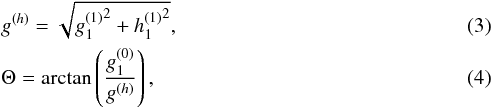 where
Θ is the inclination of the
dipole, and g(h) is amplitude of
the equatorial dipole. The components
and
determine the Carrington longitude of the equatorial dipole as
where
Θ is the inclination of the
dipole, and g(h) is amplitude of
the equatorial dipole. The components
and
determine the Carrington longitude of the equatorial dipole as
 , its azimuth
Λ is calculated as the sum of
the Carrington longitude and the phase offset, ΦCar. Figures 2 and
3a,b show the evolution of the components of the
dipolar field of the Sun.
, its azimuth
Λ is calculated as the sum of
the Carrington longitude and the phase offset, ΦCar. Figures 2 and
3a,b show the evolution of the components of the
dipolar field of the Sun.
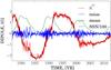 |
Fig. 2 Temporal evolution of the axisymmetric component of the solar magnetic dipole (red), its Gaussian filtering with a 1-year window (black) and the residual noise (blue), compared with sunspot number. |
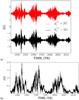 |
Fig. 3 a) Components of the solar equatorial dipole; b) Amplitude of the equatorial dipole. |
4. A dynamo model
Our idea is to start with a simple axisymmetric dynamo model and to add small-scale
nonaxisymmetric injections of poloidal magnetic field, distributed randomly in area over the
whole surface of the sphere. For the underlying (axisymmetric) dynamo model we use an
extension of the 1D Parker model, as described by Moss et
al. (2004), see also Moss et al. (2008). The
governing equations for the toroidal field B(θ) and potential A(θ) for the
poloidal field are 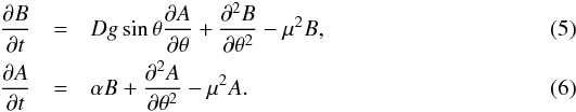 Here
θ is the
polar angle, the factor μ is introduced to represent radial diffusion, and we
take μ = 3 as
appropriate for a dynamo region of about 30% in radius. The factor g(θ) is introduced to allow a
representation of latitudinal variations in the rotation law (we put g = 1) and set the dynamo
number D = −
103. Of course it would be possible to use a more
sophisticated, two-dimensional, dynamo model. However we are not here studying details of
the overall field behaviour as a function of radius, but rather we only need a mechanism to
produce approximately sinusoidal variations of radial field at the surface.
Here
θ is the
polar angle, the factor μ is introduced to represent radial diffusion, and we
take μ = 3 as
appropriate for a dynamo region of about 30% in radius. The factor g(θ) is introduced to allow a
representation of latitudinal variations in the rotation law (we put g = 1) and set the dynamo
number D = −
103. Of course it would be possible to use a more
sophisticated, two-dimensional, dynamo model. However we are not here studying details of
the overall field behaviour as a function of radius, but rather we only need a mechanism to
produce approximately sinusoidal variations of radial field at the surface.
Once our model has settled to a regular oscillatory behaviour we map the axisymmetric field from the mean field dynamo on to the surface of a sphere. Then we add, at fixed time intervals dtinj, co-rotating patches of radial field, strength Binj of arbitrary sign, in circular regions at randomly located positions on the surface of the sphere. In the models described, these regions are of radius 20 − 30°. They are intended to represent injections of field from solar active regions – we are only interested in the resulting contributions to the global poloidal field. The resulting global poloidal field is thus nonaxisymmetric, being the sum of the symmetric dynamo generated field and the injections which are random in longitude (and in latitude). In our modelling the injected field is just added formally to the poloidal field output from Eqs. (5), (6) – the injected field is not input back into the dynamo equations. We can justify this procedure by noting that the dynamo is the result of processes occurring deep within the Sun, and can hardly be affected by the superficial phenomena associated with surface activity (“the tail does not wag the dog”).
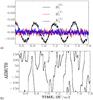 |
Fig. 4 a) Evolution of the magnetic dipole components from the model data (with time-independent amplitude of poloidal field injections, which are of arbitrary sign). b) Evolution of azimuth (see comments in the text).If the half-period (0.176) of the oscillations in panel a) is identified with the 11 yr sunspot cycle, then the time unit is about 62.5 yr. |
The injected field has strength of order the maximum dynamo poloidal field and decays with time constant tdec. The code allows multiple spots to coexist, with each generated successively after the fixed interval dtinj. If appropriate, we can modulate the injection amplitude with the phase of solar cycle. The evolution of the dipole components for a typical realization of the model is illustrated in Fig. 4a. The result is not very sensitive to the input parameters. The azimuth of the dipole is random, because of the nature of the field injection mechanism. It is determined by the position of the instantaneous dipole, which in turn is given by the most recent surface field fluctuations. The evolution of the toroidal field follows the evolution of the axial dipole with a phase shift of about π/ 2, and with amplitude of the toroidal field larger by a factor of about 40 compared to the poloidal. (This ratio could easily be adjusted by changing the parameters in Eqs. (5), (6), without changing our general conclusions.) Figure 4b illustrates the evolution of azimuth, smoothed using a Gaussian filter with a window which corresponds to one year in the model. Any apparent correlation in the evolutionary paths in Fig. 6 appears to be coincidental.
5. Results
5.1. Basic analysis of the data
For the purpose of analysis we have to separate the mean and fluctuating parts of the
field and then do the same for the inclination and azimuth of the dipole. For the
axisymmetric part of the dipole, which is represented by
,
this can be done by suitable filtering of the data in the time series. We use a Gaussian
filter with a one year window, which is often used in analysis of the sunspot data set
Hathaway (2009). Figure 2 shows the evolution of , its
mean and noise components, and the smoothed sunspot number as given by the SIDC (2010) data base. Note that the noise is
not the fluctuating part of the field (as defined in Sect. 4), but the numerical residual after data analysis.
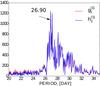 |
Fig. 5 Spectrum of the equatorial dipole components. |
Now we move to the analysis of the behaviour of the equatorial dipole, and our first aim
is to determine the rotation rate of this dipole. For this purpose we determine Fourier
spectra of
and
using the standard fast Fourier transform (FFT) routines provided by Scientific
Python1. Figure 5 shows the result. Very similar spectra were found earlier by Svalgaard & Wilcox (1975) and Kotov & Levitskii (1983) from analysis of the
rotation of the interplanetary magnetic field. We see that the spectra have peaks in a
range of synodic rotation periods between 26 and 30 days, including the Carrington period
of 27.2753 days. We recall that the synodic rotation period refers to motion as observed
from Earth. Our interpretation of the plot is that the azimuthal dipole field is, of
course, not just white noise and that its memory is sufficiently long to feel the dipole
rotation and to enable identification of at least the main peak in the spectra, which
corresponds to the rotation period P = 26.90 days. The scatter of the periods in Fig.
5 could be a consequence of the differential
rotation. In this paper we restrict our analysis to a particular mode with period
P = 26.90
days.
 |
Fig. 6 a) Transformed components of the equatorial dipole, rotation period P = 26.90 days; b) azimuth of the equatorial dipole in the frame rotating with Carrington period P = 27.253 days (upper curve) and azimuth for the mode P = 26.90 days (lower curve). |
We perform a filtering of the azimuthal dipole data in the frame rotating with the period
P = 26.90
days using the following transformation  (7)Figure
6a shows evolution of the components obtained in
result of this transformation for the case Ω =
2π/P,
P = 26.90
days. Similar results can be obtained for other periods from the given range. The
amplitude of the equatorial dipole remains the same under transformation.
(7)Figure
6a shows evolution of the components obtained in
result of this transformation for the case Ω =
2π/P,
P = 26.90
days. Similar results can be obtained for other periods from the given range. The
amplitude of the equatorial dipole remains the same under transformation.
Figure 6b shows how different the azimuth can be if we follow the original equatorial dipole components (Fig. 3) and the components of the mode P = 26.90 days. For example, we observe the quasi-regular large-scale fluctuation of this mode during the descending phase of cycle 23, when the mode was permanently visible around longitude 260° for an interval of about 3 years starting around the year 2002. The existence of such events is also suggested by results of thorough period analysis (see, e.g., Berdyugina et al. 2006). We have to stress that the our particular procedure of analysis is employed because of our restriction to consideration of the first three modes of the decomposition given by the definitions of azimuth from Eq. (1). The azimuth can be uncertain if the signal has a complicated spectrum like that shown by Fig. 5. In the literature, the reader can find some alternative possibilities for determination of the azimuth of the solar dipole (e.g. Noonoj & Kuklin 1988; de Patoul et al. 2013). However, our method allows direct comparison of results with predictions of the dynamo models.
The nonaxisymmetric modes have the largest variations in time. Using the modes in the rotating coordinate frame we can define the inclination and the azimuth of dipole for the same reference frame. For the remainder of our illustrations we use the mode corresponding to the period P = 26.90 days. This value corresponds to the position of the highest peak in Fig. 5. Clearly, in our definition the azimuth of the global dipole has an arbitrary zero point. On the other hand, it is well-known that the given characteristics of the large-scale magnetic field of the Sun trace the sectorial structure of the interplanetary magnetic field in the heliosphere Hoeksema (1995). A problem in determination of the global dipole azimuth is that the two-sector structure, which is observed during much of the cycle, changes to a four sector structure during the maxima of the sunspot cycle. The sectorial structure reflects the total contribution of all the non-axisymmetric modes. It can be used for the azimuth determination only during the phases when the two-sector structure dominates.
 |
Fig. 7 Evolution of the large-scale dipolar magnetic field components plotted with the sunspot number data. |
We show the long-term evolution of the magnitude of the total dipole strength of the solar field in Fig. 7, together with the sunspot number data. The Sun currently appears to be presenting rather atypical behaviour in the context of the last century or so. The ongoing decline in activity emphasizes that we are not dealing with a strictly periodic system and that our modelling, by assuming an underlying regular periodicity, can only hope to give a partial representation.
5.2. Axial dipole data
We calculate the rms value of the noise δd, the amplitude of the magnetic dipole cycle
variations  and its ratio
  ,
both for the observations (d is estimated for cycle 22) and the model to get the
following results. The observations give δd = 0.24,
,
both for the observations (d is estimated for cycle 22) and the model to get the
following results. The observations give δd = 0.24,  ,
,
 . For the amplitude of the
observed equatorial dipole we get similar results (see Fig. 3b and Fig. 7). Here magnetic field is
normalized to the solar radius R and magnetic moment is measured in units of Gauss
R3. For illustration, we compare with one
of our models which has a half period (corresponding to the 11 yr sunspot cycle) of 0.176
in our dimensionless units, dtinj = 0.0015 =
dtdec, and 5 spots are simultaneously
present (although by the time a spot is removed from the simulation, it has been present
for 5 decay times, and so its field is essentially reduced to zero). The model gives
δd =
0.00085,
. For the amplitude of the
observed equatorial dipole we get similar results (see Fig. 3b and Fig. 7). Here magnetic field is
normalized to the solar radius R and magnetic moment is measured in units of Gauss
R3. For illustration, we compare with one
of our models which has a half period (corresponding to the 11 yr sunspot cycle) of 0.176
in our dimensionless units, dtinj = 0.0015 =
dtdec, and 5 spots are simultaneously
present (although by the time a spot is removed from the simulation, it has been present
for 5 decay times, and so its field is essentially reduced to zero). The model gives
δd =
0.00085,  ,
,
 . Here magnetic field is
measured in units of the equipartition magnetic field. For an order of magnitude estimate,
we assume that the magnetic field unit in the model corresponds to 103 G (typical field strength of
sunspots) and then normalize to the solar radius. This gives δ = 15 Gauss
R3 and δd = 0.85 Gauss
R3. Taking into account the very crude
nature of the model, this seems to be in reasonable agreement with observations. In
physical units, the injection interval dtinj is about 0.094 yr
(ca 1.1 months), which we chose rather arbitrarily to be equal to the decay time
tdec.
. Here magnetic field is
measured in units of the equipartition magnetic field. For an order of magnitude estimate,
we assume that the magnetic field unit in the model corresponds to 103 G (typical field strength of
sunspots) and then normalize to the solar radius. This gives δ = 15 Gauss
R3 and δd = 0.85 Gauss
R3. Taking into account the very crude
nature of the model, this seems to be in reasonable agreement with observations. In
physical units, the injection interval dtinj is about 0.094 yr
(ca 1.1 months), which we chose rather arbitrarily to be equal to the decay time
tdec.
We conclude that the model produces fluctuations of the magnetic dipole that are comparable to those found in the observations. The general nature of the results was not very sensitive to the choice of parameters, provided that the interval between injections is not too long or very short, or that the injected field strength is not much larger or smaller than the maximum dipole field strength produced by the dynamo. The results are quite insensitive to tdec, provided that it is not very long, or to the number of spots present provided that dtinj and dtdec are not very different in magnitude.
We can estimate the relative duration of the reversal epoch t∗ as follows.
If the cyclic behaviour is sinusoidal, we can estimate the time during which
 is lower than δd. A simple calculation gives
 , and for an 11-year cycle
t∗ ≈
4 month.
, and for an 11-year cycle
t∗ ≈
4 month.
The autocorrelation function of the noise is presented in Fig. 8. The correlation time of the fluctuations can be estimated from the plot as τcor ≈ 0.18 yr = 65 d ≈ 2 months, i.e. about half the duration of the reversal epoch. Note, that parameters of fluctuations of the axial dipole and the amplitude of the equatorial dipole are rather similar.
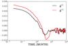 |
Fig. 8 Auto-correlation function of the magnetic dipole fluctuations (mean values are subtracted). |
We estimate 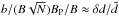 (here B is the mean magnetic
field field and BP its poloidal component) following Eq.
(1) of Moss et al. (2013), where B is the large-scale
magnetic field strength in the near-surface layers within the Sun, b is the corresponding
strength of magnetic fluctuations and N is number of convective cells in the domain of
dynamo action. Again following Moss et al. (2013),
we take as a crude estimate N
= 103 and BP/B ≈
0.1 and arrive at an estimate b/B =
2, which is more or less in agreement with the estimate obtained by
Sokoloff & Khlystova (2010) from
statistics of the sunspot groups that violate the Hale polarity law.
(here B is the mean magnetic
field field and BP its poloidal component) following Eq.
(1) of Moss et al. (2013), where B is the large-scale
magnetic field strength in the near-surface layers within the Sun, b is the corresponding
strength of magnetic fluctuations and N is number of convective cells in the domain of
dynamo action. Again following Moss et al. (2013),
we take as a crude estimate N
= 103 and BP/B ≈
0.1 and arrive at an estimate b/B =
2, which is more or less in agreement with the estimate obtained by
Sokoloff & Khlystova (2010) from
statistics of the sunspot groups that violate the Hale polarity law.
5.3. Direction of the magnetic dipole at the epoch of reversal
We can follow the evolution of the total magnetic dipole during the epoch of reversal by plotting the position of the end of the dipole vector as a point on a sphere of unit radius (Fig. 9a). We conclude that the reversal track for the model (Fig. 9c) is quite similar to that deduced from observations. Of course, a shorter filtering time gives a more complicated trajectory for the dipole. We give an alternative presentation of the dipole track in Fig. 10.
 |
Fig. 9 Track of the pole of the magnetic dipole on a sphere of unit radius. a) WSO data using a Gaussian filter with a one-year window for the model described in Fig. 4; b) same for the half-year window; c) same for the model – see Fig. 4 – which, in contrast to the data, covers an interval with 6 reversals of the global dipole. |
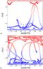 |
Fig. 10 Track of the pole of the magnetic dipole in the θ–λ plane: a) WSO data, b) the same for the model (Fig. 4) which, in contrast to the 4 reversals in the WSO data, covers an interval with 6 reversals of the global dipole. |
We find that the trajectories of the pole of the magnetic dipole depend on the method of smoothing applied to the WSO data as well as for the model data. These plots are quite similar to those shown in Fig. 9b and we do not present them here. Using the model data, we demonstrated that the longitude of reversal tracks is distributed on the sphere quite randomly. Unfortunately, there are no corresponding long-term observational data to confirm this point observationally.
5.4. Cyclic evolution of the amplitude of magnetic fluctuations
According to the interpretation of the observational data suggested, the equatorial magnetic dipole is a large-scale manifestation of magnetic fluctuations. A notable feature of the plots describing the equatorial dipole (Figs. 3, 6) is that the amplitude of the noise is modulated with the solar cycle period. We did not include such a feature in our model, so quite naturally the plot for the equatorial dipole for the model data (Fig. 4) does not show such an effect. If we include modulation of the fluctuations with the amplitude of the toroidal field variations, the desired modulation of the equatorial dipole appears.
We conclude that the rms of the solar magnetic fluctuations has an 11-year periodicity. We find that this modulation survives if we introduce artificially a long-term evolution of the cycle amplitude, as has occurred during recent solar cycles (we omit the plot for the sake of brevity). We note that cyclic behaviour of the equatorial dipole was mentioned previously by Hoeksema (1995) and Obridko & Livshits (2006).
6. Discussion and conclusions
Our analysis of the observational data, and comparison with a simple model of the solar dynamo, confirm that non-zero nonaxisymmetric values of the total magnetic dipole at the epoch of solar magnetic reversal are consistent with a large-scale contribution from fluctuations of the solar surface magnetic field, as discussed by Moss et al. (2013). We envisage that these fluctuations, connected loosely to active regions, are driven by an instability of the underlying layers.
The analysis gives an estimate for the ratio of the rms value of the fluctuation to the amplitude of cyclic variations of the mean solar field of b/B ≈ 2. This estimate is independent of the estimate of Sokoloff & Khlystova (2010), obtained from the statistics of sunspot groups that do not follow the Hale polarity law. These estimates differ by a factor of about 2, which appears quite satisfactory given that the amplitude of solar cycle varies substantially from cycle to cycle, and that the estimates come from analyses of quite different data.
The random nature of the orientation of the solar magnetic dipole during the epoch of reversal is clearly visible from the trajectories of the pole of the magnetic dipole on the unit sphere (Fig. 9c). On the other hand, the epoch of reversal occupies a relatively small part of the solar cycle (about 4 months only). The duration of the reversal epoch is estimated as the time during which the fluctuating part of the dipole is larger than the mean-field contribution. In comparison, the memory time for the dipole fluctuations is estimated as about 2 months, i.e. about half the duration of the reversal epoch. This is why the dipole trajectory is far from just being noise, and some traces of regular behaviour are visible in the trajectory during a given reversal. This might be instructive for understanding of the phenomenon of active longitudes (e.g. Usoskin et al. 2007, and references therein).
Our analysis gives further important information relevant to studies of the solar dynamo. We see that magnetic fluctuations are cyclically modulated. This means that they (at least mainly) originate in the periodic global dynamo action, rather than from small-scale dynamo action, as was suggested by Goode et al. (2012) and Abramenko (2013). Possibly this is because active regions are generated more readily in the parts of the cycle where toroidal fields are stronger – recall that the axisymmetric poloidal field is out of phase with the dynamo generated toroidal field. In other words, we confirm here the interpretation of Stenflo (2013) that a local dynamo does not give a significant contribution to the observed small-scale flux. Following this interpretation however, based on other observational data, we infer that, as far as we can confirm from the observations available, solar magnetic activity is a result of a single physical process which simultaneously generates the solar activity cycle as well as the magnetic fluctuations. We do not exclude in principle the possibility that an additional dynamo excitation mechanism for small-scale magnetic field is active somewhere in the solar interior. However we are unable to isolate its manifestations from the general cyclic behaviour associated with the main driver of solar magnetic activity.
One more important point is that the small-scale magnetic fluctuations considered here result in weak nonaxisymmetric magnetic field components, as demonstrated by the equatorial dipole data (Figs. 3, 6). An additional illustration of this fact is given in Fig. 7 which plots the large-scale total dipole component of the solar activity, including both the axisymmetric and nonaxisymmetric parts. We see that the nonaxisymmetric components are stronger during maxima of sunspot activity, i.e. they are associated with the toroidal magnetic field. The lifetime of bursts of nonaxisymmetric components is of order 1 year. Any such large-scale components could be described by standard mean-field dynamo equations. Moss et al. (2013) estimated the lifetime of such nonaxisymmetric bursts as about 1 year, in reasonable agreement with observations.
Our interpretation is that the nonaxisymmetric magnetic field components appear as a result of decay of the large-scale toroidal magnetic field. The typical correlation time of the nonaxisymmetric modes is estimated to be around 1 year. This agrees with results of the recent analysis of rotation of solar active regions made by Pelt et al. (2010). They, following Krause & Rädler (1980), suggested the existence of non-oscillatory nonaxisymmetric modes which rotate rigidly with an angular velocity that is different from the overall rotation period. These modes are coupled to the global toroidal field and affected by differential rotation. This is consistent with the results presented in Fig. 5. Note that wavelet analysis by Mordvinov & Plyusnina (2000) reveals that nonaxisymmetric modes with different periods of rotations are excited during different epochs of the solar cycle, e.g. the mode with P = 26.9 days is present during the decaying phase of activity, while modes with periods around 28 days are present during the rising phase of the solar cycle (cf. Fig. 6b). Perhaps an equally valid interpretation is to link the rotation rates to the rotation rates of the remnant flux patterns. A more complicated approach might include the possibility of azimuthal dynamo wave excitation in spherical shell convection (Cole et al. 2014). Note, the rotational periods of the emerging nonaxisymmetric fields can be related to the “new magnetic flux” which might originate in a subsurface shear layer – Benevolenskaya et al. (1999). This is compatible with a distributed dynamo operating in the bulk of the convection zone and being shaped by the subsurface shear layer (Brandenburg 2005; Pipin & Kosovichev 2011).
Obviously, our interpretation does not exclude the possibility that occasionally the equatorial magnetic dipole might vanish simultaneously with the strength of the axial dipole (which is part of the mean field) passing through zero during the course of an reversal. In such a case, at some instant during the reversal the total dipole will vanish. Remarkably (cf. Fig. 7), this seems to be happening just now (Obridko 2013). Of course, there are details of the data that we have not analyzed, which could affect our conclusions. These include, for example, the study of effects of the higher order components of the decomposition Eq. (1) on reversals of polar field. However, such a study goes beyond the simple dynamo model discussed in this paper.
In summary, we have presented a simple heuristic model – basically a cartoon – to illustrate a mechanism to reproduce the behaviour of the solar dipole during reversals. We have necessarily made a number of more-or-less arbitrary – but reasonable – assumptions. Our principle conclusion is that a model of this sort can quite satisfactorily represent the observed phenomena during a reversal. The mechanism seems quite robust, and our results quantitatively support the idea proposed by Moss et al. (2013). Thus we feel confident that it captures the essence of the solar behaviour without performing excessive fine tuning. Moreover, we find that the detailed observational data concerning solar dipole reversals have, perhaps rather unexpectedly, the potential to reveal much about dynamo action in the solar interior. Clearly, there is considerable scope for a more detailed analysis of a more sophisticated model.
Acknowledgments
V.P. and D.S. are grateful to RFBR for financial support under grant 12-02-00170-a. Useful discussions with V.N. Obridko are acknowledged. An anonymous referee made a number of valuable comments which improved the text.
References
- Abramenko, V. I. 2013, in IAU Symp. 294, eds. A. G. Kosovichev, E. de Gouveia Dal Pino, & Y. Yan, 289 [Google Scholar]
- Benevolenskaya, E. E., Hoeksema, J. T., Kosovichev, A. G., & Scherrer, P. H. 1999, ApJ, 517, L163 [NASA ADS] [CrossRef] [Google Scholar]
- Berdyugina, S. V., Moss, D., Sokoloff, D. D., & Usoskin, I. G. 2006, A&A, 445, 703 [NASA ADS] [CrossRef] [EDP Sciences] [Google Scholar]
- Brandenburg, A. 2005, ApJ, 625, 539 [Google Scholar]
- Brown, B. P., Miesch, M. S., Browning, M. K., Brun, A. S., & Toomre, J. 2011, ApJ, 731, 69 [NASA ADS] [CrossRef] [Google Scholar]
- Choudhuri, A. R. 2008, Adv. Space Res., 41, 868 [NASA ADS] [CrossRef] [Google Scholar]
- Cole, E., Käpylä, P. J., Mantere, M. J., & Brandenburg, A. 2014, ApJ, 780, L22 [NASA ADS] [CrossRef] [Google Scholar]
- de Patoul, J., Inhester, B., & Cameron, R. 2013, A&A, 558, L4 [NASA ADS] [CrossRef] [EDP Sciences] [Google Scholar]
- DeRosa, M. L., Brun, A. S., & Hoeksema, J. T. 2012, ApJ, 757, 96 [Google Scholar]
- Duvall, Jr., T. L., Wilcox, J. M., Svalgaard, L., Scherrer, P. H., & McIntosh, P. S. 1977, Sol. Phys., 55, 63 [NASA ADS] [CrossRef] [Google Scholar]
- Duvall, Jr., T. L., Scherrer, P. H., Svalgaard, L., & Wilcox, J. M. 1979, Sol. Phys., 61, 233 [NASA ADS] [CrossRef] [Google Scholar]
- Fry, C. D., Akasofu, S. I., Hoeksema, J. T. & Hakamada, K. 1985, Planet. Space Sci., 33, 915 [NASA ADS] [CrossRef] [Google Scholar]
- Goode, P. R., Abramenko, V., & Yurchyshyn, V. 2012, Phys. Scr., 86, 018402 [NASA ADS] [CrossRef] [Google Scholar]
- Hathaway, D. 2009, Space Sci. Rev., 144, 401 [NASA ADS] [CrossRef] [Google Scholar]
- Hoeksema, J. T. 1995, Space Sci. Rev., 72, 137 [Google Scholar]
- Hoeksema, J. T., & Scherrer, P. H. 1986, Sol. Phys., 105, 205 [NASA ADS] [CrossRef] [Google Scholar]
- Kotov, V. A., & Levitskii, L. S. 1983, Izvestiya Ordena Trudovogo Krasnogo Znameni Krymskoj Astrofizicheskoj Observatorii, 68, 56 [NASA ADS] [Google Scholar]
- Krause, F., & Rädler, K.-H. 1980, Mean-Field Magnetohydrodynamics and Dynamo Theory (Berlin: Akademie-Verlag) [Google Scholar]
- Livshits, I. M., & Obridko, V. N. 2006, Astr. Rep., 50, 926 [NASA ADS] [CrossRef] [Google Scholar]
- Mordvinov, A. V., & Plyusnina, L. A. 2000, Sol. Phys., 197, 1 [NASA ADS] [CrossRef] [Google Scholar]
- Moss, D., Sokoloff, D., Kuzanyan, K., & Petrov, A. 2004, Geophy. Astrophys. Fluid Dyn., 98, 257 [Google Scholar]
- Moss, D., Saar, S., & Sokoloff, D. 2008, MNRAS, 388, 416 [NASA ADS] [CrossRef] [Google Scholar]
- Moss, D., Kitchatinov, L. L., & Sokoloff, D. 2013, A&A, 550, L9 [Google Scholar]
- Noonoj, G., & Kuklin, G. V. 1988, Issledovaniia Geomagnetizmu Aeronomii i Fizike Solntsa, 79, 49 [NASA ADS] [Google Scholar]
- Obridko, V. N. 2013, All-Russian Astronomical meeting, St Petersburg, Abstract book, 2013, 202 [Google Scholar]
- Parker, E. 1955, ApJ, 122, 293 [NASA ADS] [CrossRef] [Google Scholar]
- Pelt, J., Korpi, M. J., & Tuominen, I. 2010, A&A, 513, A48 [NASA ADS] [CrossRef] [EDP Sciences] [Google Scholar]
- Pipin, V. V., & Kosovichev, A. G. 2011, ApJ, 741, 1 [NASA ADS] [CrossRef] [Google Scholar]
- Pipin, V. V., & Kosovichev, A. G. 2013, ApJ, 776, 36 [NASA ADS] [CrossRef] [Google Scholar]
- Scherrer, P. H., Wilcox, J. M., Svalgaard, L., et al. 1977, Sol. Phys., 54, 353 [NASA ADS] [CrossRef] [Google Scholar]
- SIDC. 2010, Monthly Report on the International Sunspot Number, online catalogue, http://www.sidc.be/sunspot-data/ [Google Scholar]
- Sokoloff, D., & Khlystova, A. I. 2010, Astr. Nachr., 331, 82 [Google Scholar]
- Stenflo, J. O. 2013, in IAU Symp. 294, eds. A. G. Kosovichev, E. de Gouveia Dal Pino, & Y. Yan, 119 [Google Scholar]
- Svalgaard, L., & Wilcox, J. M. 1975, Sol. Phys., 41, 461 [NASA ADS] [CrossRef] [Google Scholar]
- Usoskin, I. G., Berdyugina, S. V., Moss, D., & Sokoloff, D. D. 2007, Adv. Space Res., 40, 951 [NASA ADS] [CrossRef] [Google Scholar]
- Zhao, X., & Hoeksema, J. T. 1993, Sol. Phys., 143, 41 [NASA ADS] [CrossRef] [Google Scholar]
All Figures
|
Fig. 1 Evolution of the dipole component of the radial magnetic field as obtained from measurements at the WSO from 1976 to 2013. |
| In the text | |
|
Fig. 2 Temporal evolution of the axisymmetric component of the solar magnetic dipole (red), its Gaussian filtering with a 1-year window (black) and the residual noise (blue), compared with sunspot number. |
| In the text | |
|
Fig. 3 a) Components of the solar equatorial dipole; b) Amplitude of the equatorial dipole. |
| In the text | |
|
Fig. 4 a) Evolution of the magnetic dipole components from the model data (with time-independent amplitude of poloidal field injections, which are of arbitrary sign). b) Evolution of azimuth (see comments in the text).If the half-period (0.176) of the oscillations in panel a) is identified with the 11 yr sunspot cycle, then the time unit is about 62.5 yr. |
| In the text | |
|
Fig. 5 Spectrum of the equatorial dipole components. |
| In the text | |
|
Fig. 6 a) Transformed components of the equatorial dipole, rotation period P = 26.90 days; b) azimuth of the equatorial dipole in the frame rotating with Carrington period P = 27.253 days (upper curve) and azimuth for the mode P = 26.90 days (lower curve). |
| In the text | |
|
Fig. 7 Evolution of the large-scale dipolar magnetic field components plotted with the sunspot number data. |
| In the text | |
|
Fig. 8 Auto-correlation function of the magnetic dipole fluctuations (mean values are subtracted). |
| In the text | |
|
Fig. 9 Track of the pole of the magnetic dipole on a sphere of unit radius. a) WSO data using a Gaussian filter with a one-year window for the model described in Fig. 4; b) same for the half-year window; c) same for the model – see Fig. 4 – which, in contrast to the data, covers an interval with 6 reversals of the global dipole. |
| In the text | |
|
Fig. 10 Track of the pole of the magnetic dipole in the θ–λ plane: a) WSO data, b) the same for the model (Fig. 4) which, in contrast to the 4 reversals in the WSO data, covers an interval with 6 reversals of the global dipole. |
| In the text | |
Current usage metrics show cumulative count of Article Views (full-text article views including HTML views, PDF and ePub downloads, according to the available data) and Abstracts Views on Vision4Press platform.
Data correspond to usage on the plateform after 2015. The current usage metrics is available 48-96 hours after online publication and is updated daily on week days.
Initial download of the metrics may take a while.