© ESO, 2014

1. Introduction

When error bars or confidence intervals are reported, the reader expects them to have their frequentist meaning. Thus, a 95% confidence interval is interpreted as implying a probability of 0.95 that the true result is enclosed by that interval. Similarly, the interval defined by ± 1σ error bars is expected to include the true answer with probability 0.683. However, this frequentist ideal is often not realized. This may be the result of observers misjudging the precision of their measurements or of large measurment errors occurring more frequently than expected for a normal distribution.

Such practical issues are absent when data analysis techniques are investigated with simulations, since precision can be exactly specified and measurement errors can be assigned with random Gaussian variates, so that one might then expect a rigorous recovery of the frequentist ideal. But approximations can still compromise statistical rigour. For example, if a grid is required, confidence intervals might be affected if the grid is too coarse. In such cases, with increased computational resources, the limit as the grid steps → 0 can be closely approached and accurate results obtained.

Of more concern are approximations that compromise confidence intervals independently of any such limit. Two examples in the recent literature occur in hybrid problems – i.e., non-linear problems with a subset of linear parameters. The first example is the code EXOFAST for analysing transit and radial velocity data for stars with orbiting planets (Eastman et al. 2013). These authors note that the convergence of their Markov chain Monte Carlo (MCMC) parameter search is much faster if the exact solution for the linear parameters is introduced. However, the resulting uncertainties in the linear parameters are as much as 10 times smaller than when fitted non-linearly. Pending further research, these authors sensibly choose the inefficient option of treating all parameters as non-linear.

A similar but less extreme example arises when Bayesian estimation is applied to visual binaries (Lucy 2014; L14). When formulated in terms of the Thiele-Innes elements, the problem becomes linear in four of the seven elements. But when this linearity is exploited, coverage fractions (L14, Sect. 5.5) indicate that the standard errors of the four linear elements are too small by factors of up to 2.1.

These examples pose a statistical challenge in the analysis of orbits: How can we benefit from partial linearity without losing the frequentist properties of confidence intervals? In this paper, this challenge is addressed in its visual binary context and for both frequentist and Bayesian procedures.

2. Synthetic orbits

The paper L14 is followed closely with regard both to notation and in the creation of synthetic data.

2.1. Orbital elements

The orbit of the secondary relative to its primary is conventionally parameterized by its Campbell elements P,e,T,a,i,ω,Ω. Here P is the period, e is the eccentricity, T is a time of periastron passage, i is the inclination, ω is the longitude of periastron, and Ω is the position angle of the ascending node. However, from the standpoint of computational economy, many investigators – references in L14 Sect. 2.1 – prefer the Thiele-Innes elements. Thus, the Campbell parameter vector θ = (φ,ϑ), where φ = (P,e,τ) and ϑ = (a,i,ω,Ω), is replaced by the Thiele-Innes vector (φ,ψ), where the components of the vector ψ are the Thiele-Innes constants A,B,F,G. (Note that in the φ vector, T has been replaced by τ = T/P which by definition ∈ (0,1).)

2.2. Model binary

As in L14, the adopted model binary has the following Campbell elements:

$\begin{array}{ccc}& & {\mathit{P}}_{\mathrm{\ast }}\mathrm{=}\mathrm{100}\mathit{y}{\mathit{\tau }}_{\mathrm{\ast }}\mathrm{=}\mathrm{0.4}{\mathit{e}}_{\mathrm{\ast }}\mathrm{=}\mathrm{0.5}{\mathit{a}}_{\mathrm{\ast }}\mathrm{=}\mathrm{1}″\\ & & {\mathit{i}}_{\mathrm{\ast }}\mathrm{=}\mathrm{60}°{\mathit{\omega }}_{\mathrm{\ast }}\mathrm{=}\mathrm{250}°{\mathrm{\Omega }}_{\mathrm{\ast }}\mathrm{=}\mathrm{120}°\mathit{.}\end{array}$(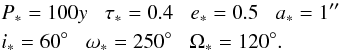1)An observing campaign for this binary is simulated by creating measured Cartesian sky coordinates $\mathrm{\left(}\begin{array}{c}{}_{\mathrm{˜}}\\ {\mathit{x}}_{\mathit{n}}\end{array}\mathit{,}\begin{array}{c}{}_{\mathrm{˜}}\\ {\mathit{y}}_{\mathit{n}}\end{array}\mathrm{\right)}$ with weights w_n at uniformly-spaced times t_n for n = 1,...,N as described in L14 Sect. 3.2. The parameters defining a campaign are f_orb, the fraction of the orbit observed, N, the number of observations, and σ, the standard error for unit weight.

For given orbital elements, the predicted orbit (x_n,y_n) is computed as described in L14 Sect. A.1, and the quality of the fit is determined by 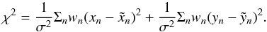${\mathit{\chi }}^{\mathrm{2}}\mathrm{=}\frac{\mathrm{1}}{{\mathit{\sigma }}^{\mathrm{2}}}{\mathrm{\Sigma }}_{\mathit{n}}{\mathit{w}}_{\mathit{n}}\mathrm{(}{\mathit{x}}_{\mathit{n}}\mathrm{-}\begin{array}{c}\mathrm{˜}\\ {\mathit{x}}_{\mathit{n}}\end{array}{\mathrm{)}}^{\mathrm{2}}\mathrm{+}\frac{\mathrm{1}}{{\mathit{\sigma }}^{\mathrm{2}}}{\mathrm{\Sigma }}_{\mathit{n}}{\mathit{w}}_{\mathit{n}}\mathrm{(}{\mathit{y}}_{\mathit{n}}\mathrm{-}\begin{array}{c}\mathrm{˜}\\ {\mathit{y}}_{\mathit{n}}\end{array}{\mathrm{)}}^{\mathrm{2}}\mathit{.}$(2)

3. Minimum-χ² estimation

The conventional (frequentist) approach to orbit-fitting is the method of least squares – i.e., finding the elements that minimize χ². When the problem is non-linear, the search for the minimum typically involves successive differential corrections obtained from linearized equations, starting with an initial guess. However, in treating incomplete orbits and imprecise data, it is preferable to find ${\mathit{\chi }}_{\min }^{\mathrm{2}}\mathrm{=}{\mathit{\chi }}^{\mathrm{2}}\mathrm{\left(}\mathit{\theta ̂}\mathrm{\right)}$ by means of a grid search (e.g., Hartkopf et al. 1989; Schaefer et al. 2006) and then to derive confidence intervals from constant χ² “surfaces” in parameter space (e.g., Press et al. 1992, Chap. 15.6; James 2006, Chap. 9.1.2).

3.1. Grid search

In a brute force approach to finding , values of χ² would be computed throughout a 7D grid. Confidence intervals for the elements would then be derived from projections of the 7D volume defined by the inequality 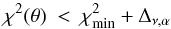${\mathit{\chi }}^{\mathrm{2}}\mathrm{\left(}\mathit{\theta }\mathrm{\right)}\mathit{<}{\mathit{\chi }}_{\min }^{\mathrm{2}}\mathrm{+}{\mathrm{\Delta }}_{\mathit{\nu ,\alpha }}$(3)where the constant Δ_ν,α is detemined by ν, the number of degrees of freedom and α, the desired confidence level. With a typical 100 steps for each dimension, the brute force method requires χ² to be evaluated at ~10¹⁴ grid points. However, if the linearity with respect to the Thiele-Innes elements can be exploited, χ² is only required at ~10⁶ grid points. This potential reduction by a factor of ~10⁸ in the number of computed orbits is a powerful incentive to solve the challenge posed in Sect. 1.

On the assumption that linearity can be exploited, grid searches in this paper are restricted to the φ-elements P,e,τ. The grid is defined by taking constant steps spanning the intervals (log P_L,log P_U),(e_L,e_U),(τ_L,τ_U). The grid cells are labelled (i,j,k) and the φ-elements at the mid-points are log P_i,e_j,τ_k. With these values fixed, ${\mathit{\chi }}_{\mathit{ijk}}^{\mathrm{2}}$ is a function of ψ = (A,B,F,G) and has its minimum value $\mathit{\chi ̂}\begin{array}{c}\mathrm{2}\\ \mathit{ijk}\end{array}$ at the point given by Eqs. (A.7) in L14.

Because ${\mathit{\chi }}_{\mathit{ijk}}^{\mathrm{2}}\mathrm{\ge }\mathit{\chi ̂}\begin{array}{c}\mathrm{2}\\ \mathit{ijk}\end{array}$, it follows that nowhere in (φ_ijk,ψ)-space is ${\mathit{\chi }}_{\mathit{ijk}}^{\mathrm{2}}\mathrm{\left(}\mathit{\psi }\mathrm{\right)}$ less than the minimum value found in the 3D search. Accordingly, in the limit of vanishingly small grid steps, 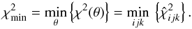${\mathit{\chi }}_{\min }^{\mathrm{2}}\mathrm{=}\underset{\mathit{\theta }}{\min }\mathrm{\left\{}{\mathit{\chi }}^{\mathrm{2}}\mathrm{\right(}\mathit{\theta }{\mathrm{\left)}}^{\mathrm{\right\}}}\mathrm{=}\underset{\mathit{ijk}}{\min }\mathrm{\{}\mathit{\chi ̂}{\begin{array}{c}\mathrm{2}\\ \mathit{ijk}\end{array}}^{\mathrm{\}}}\mathit{.}$(4)Thus, as has long been understood (e.g, Hartkopf et al. 1989), the minimum-χ² elements can be found with a grid search restricted to the non-linear elements.

3.2. Approximate confidence intervals

With determined, the calculation of confidence intervals requires projections of , the volume in θ-space defined by Eq. (3). In the absence of a 7D grid, a possible approach is to derive approximate confidence intervals from projections of the 3D grid points satisfying Eq. (3) – i.e., from projections of the domain comprising grid points such that $\mathit{\chi ̂}\begin{array}{c}\mathrm{2}\\ \mathit{ijk}\end{array}\mathit{<}{\mathit{\chi }}_{\min }^{\mathrm{2}}\mathrm{+}{\mathrm{\Delta }}_{\mathit{\nu ,\alpha }}\mathit{.}$(5)This derivation of confidence intervals has exploited linearity since it relies on obtaining and therefore also $\mathit{\chi ̂}\begin{array}{c}\mathrm{2}\\ \mathit{ijk}\end{array}$ without iteration. However, every point also satisfies Eq. (3), so that . Accordingly, these approximate intervals will always be enclosed within the true intervals and so may give a misleading impression of the elements’ precision.

3.3. Accurate confidence intervals

An asymptotically rigorous calculation proceeds as follows: first, since ${\mathit{\chi }}_{\mathit{ijk}}^{\mathrm{2}}\mathrm{\left(}\mathit{\psi }\mathrm{\right)}\mathrm{\ge }\mathit{\chi ̂}\begin{array}{c}\mathrm{2}\\ \mathit{ijk}\end{array}$, the points (φ_ijk,ψ) are all exterior to when . Thus grid points are no longer of interest.

Now consider a point . A point in the ψ-space attached to φ_ijk has a χ² higher than the least squares value at φ_ijk by the amount $\mathit{\delta }{\mathit{\chi }}_{\mathit{ijk}}^{\mathrm{2}}\mathrm{=}{\mathit{\chi }}_{\mathit{ijk}}^{\mathrm{2}}\mathrm{-}\mathit{\chi ̂}\begin{array}{c}\mathrm{2}\\ \mathit{ijk}\end{array}\mathit{.}$(6)This point is on the 6D surface of the volume if $\mathit{\delta }{\mathit{\chi }}_{\mathit{ijk}}^{\mathrm{2}}\mathrm{=}{\mathrm{\Delta }}_{\mathit{\nu ,\alpha }}\mathrm{-}\mathrm{(}\mathit{\chi ̂}\begin{array}{c}\mathrm{2}\\ \mathit{ijk}\end{array}\mathrm{-}{{\mathit{\chi }}_{\min }^{\mathrm{2}}}^{\mathrm{)}}\mathit{.}$(7)The contribution to arising from the grid point (i,j,k) can therefore be obtained by randomly sampling the attached ψ-space subject to this constraint on $\mathit{\delta }{\mathit{\chi }}_{\mathit{ijk}}^{\mathrm{2}}$. The superposition of these contributions from all then maps out , and the projections of give the desired confidence intervals.

If is the number of random points ψ_ℓ on generated at each φ_ijk, the ensemble of generated points (φ_ijk,ψ_ℓ) becomes an exact representation of in the limits and grid steps → 0. In other words, in these limits no finite surface element would be missed by the random sampling.

The merits of this procedure are the following: 1) The random sampling on does not require further orbits to be calculated; 2) in contrast to acceptance-rejection methods common in Monte Carlo sampling, all points are accepted; and 3) in contrast to the brute force approach, no points are computed either interior or exterior to .

3.4. An example

To illustrate this calculation of confidence intervals, the model binary with elements given in Eq. (1) is observed in a campaign with parameters f_orb = 0.6,N = 15,σ = 0″05. The initial 3D search for ${\mathit{\chi }}_{\min }^{\mathrm{2}}$ is on a coarse 100³ grid spanning the intervals (1,4),(0,1),(0,1) in log P,e,τ, respectively. Given the resulting initial estimate of ${\mathit{\chi }}_{\min }^{\mathrm{2}}$, the search boundaries are pruned in such a way that no point with ${\mathit{\chi }}^{\mathrm{2}}\mathit{<}{\mathit{\chi }}_{\min }^{\mathrm{2}}\mathrm{+}\mathrm{25}$ is excluded, and then a new 100³ grid is computed. The resulting ${\mathit{\chi }}_{\min }^{\mathrm{2}}$ and its location are then slightly improved by making small random displacements and acceping those that reduce χ².

An investigator selects the confidence intervals of interest by specifying ν and α. Here we take α = 0.683, corresponding to ± 1σ limits, and ν = 1, thus computing confidence intervals for each element individually – i.e., independently of the other elements. With these choices, Δ_ν,α = 1. For ± 2σ limits, α = 0.954 and Δ_ν,α = 4.

With Δ_ν,α = 1, the refined grid has 506 points satisfying Eq. (5). These define and, as described in Sect. 3.2, approximate confidence intervals are obtained from projections of . The details are as follows: At each point , the least squares values are available from the grid search. From these, the Campbell elements are calulated as described in Sect. A4 of L14. Thus the Campbell elements θ_ijk are known at every point and the projections of this ensemble give the ± 1σ intervals. Figure 1 illustrates this procedure. The (log a,i)-projection of the θ_ijk vectors is plotted as are the resulting ± 1σ limits.

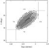Fig. 1 Approximate confidence intervals. The ensemble of orbit vectors with $\mathit{\chi ̂}\begin{array}{c}\mathrm{2}\\ \mathit{ijk}\end{array}\mathit{<}{\mathit{\chi }}_{\min }^{\mathrm{2}}\mathrm{+}\mathrm{1}$ is projected on to the (log a,i)-plane. The ± 1σ bounds for each coordinate are indicated. The 506 grid points φijk define the domain .

Now, for the same observed orbit $\mathrm{\left(}\begin{array}{c}{}_{\mathrm{˜}}\\ {\mathit{x}}_{\mathit{n}}\end{array}\mathit{,}\begin{array}{c}{}_{\mathrm{˜}}\\ {\mathit{y}}_{\mathit{n}}\end{array}\mathrm{\right)}$ and with the same refined grid, accurate ± 1σ intervals are computed according to the procedure of Sect. 3.3. At each of the 506 grid points ∈, random points on are calculated as described in Sect. A.5. These points ψ_ℓ are such that ${\mathit{\chi }}^{\mathrm{2}}\mathrm{\left(}{\mathit{\psi }}_{\mathit{\ell }}\mathrm{\right)}\mathrm{=}{\mathit{\chi }}_{\min }^{\mathrm{2}}\mathrm{+}\mathrm{1}$. For each ψ_ℓ, the corresponding Campbell elements are then derived as described in Sect. A.4 of L14. The final result is 2530 vectors . The projections of give the desired ± 1σ limits. Figure 2 illustrates this step by again projecting the cloud of points on to the (log a,i)-plane.

Because Figs. 1 and 2 refer to the same orbit and are plotted to the same scale, we see immediately that, as anticipated in Sect. 3.2, the approximate ± 1σ intervals are enclosed by the accurate intervals. The ratios accurate:approximate are 1.4 for log a and 1.9 for i.

A point to note from Figs. 1 and 2 is that with finite samples, the derived confidence limits will always be underestimates. In the above example, increasing from 5 to 500 increases the confidence intervals for log a and i by additional factors of 1.045 and 1.055, respectively. Convergence experiments indicate that sufficient accuracy is achieved with .

The error bars derived with these procedures for a quantity Q are in general not symmetric about its minimum-χ² value. Accordingly, in testing these procedures, attention is focussed not on error bars but on confidence intervals (Q_L,Q_U).

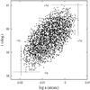Fig. 2 Accurate confidence limits. The ensemble of orbit vectors – i.e., with ${\mathit{\chi }}_{\mathit{\ell }}^{\mathrm{2}}\mathrm{=}{\mathit{\chi }}_{\min }^{\mathrm{2}}\mathrm{+}\mathrm{1}$ – is projected on to the (log a,i)-plane. The ± 1σ bounds for each coordinate are indicated. Each of the 506 grid points gives rise to points on .

3.5. Coverage fractions

Confidence intervals calculated as described in Sect. 3.3 are claimed to be asymptotically rigorous. This implies that, with a fine enough grid and a sufficiently large , coverage fractions will be close to their frequentist values. To test this, two experiments similar to those in Sect. 5.5 of L14 are now reported. In each experiment, the example of Sect. 3.4 is repeated 10 000 times with independent realizations $\mathrm{\left(}\begin{array}{c}{}_{\mathrm{˜}}\\ {\mathit{x}}_{\mathit{n}}\end{array}\mathit{,}\begin{array}{c}{}_{\mathrm{˜}}\\ {\mathit{y}}_{\mathit{n}}\end{array}\mathrm{\right)}$ of the observed orbit. For each trial, confidence intervals are computed for various quantities Q, and an interval is counted as a success if Q_L<Q_exact<Q_U. The quanties Q are the Campbell elements plus the mass estimator ℳ defined in Eq. (17) of L14.

The approximate and accurate intervals of Sect. 3.2 and Sect. 3.3 – now with – are investigated in experiments i and ii, respectively. In each experiment, both ± 1σ and ± 2σ intervals are tested.

The results are reported in Table 1. From experiment i, we see that the approximate confidence intervals are too small by factors of up to 1.9 for the ± 1σ intervals and up to 1.4 for the ± 2σ intervals. In contrast, the results for experiment ii are close to ideal. Specifically, to within errors, the ± 2σ coverage fractions match the frequentist value. On the other hand, the ± 1σ coverage fractions fall short by the inconsequential factor of 1.016, indicating the need for a somewhat larger .

These results support the claim that the procedure developed in Sect. 3.3 is asymptotically rigorous. Moreover, the additional computational burden is negligible: experiment ii required a mere 11% more computer time than experiment i.

4. Bayesian estimation

In this section, the Bayesian treatment of L14 is modified to eliminate its dependence on the profile likelihood – Eq. (3) in L14.

4.1. Posterior density

The posterior probability density function (PDF) at (φ,ψ) given data D is $\mathrm{\Lambda }\mathrm{\left(}\mathit{\phi ,\psi }\mathrm{\right|}\mathit{D}\mathrm{)}\mathrm{\propto }\mathrm{ℒ}\mathrm{(}\mathit{\phi ,\psi }\mathrm{\left|}\mathit{D}\mathrm{\right)}\mathit{\pi }\mathrm{\left(}\mathit{\phi ,\psi }\mathrm{\right)}$(8)where ℒ is the likelihood of (φ,ψ) given D, and π(φ,ψ) is a PDF that quantifies the investigator’s prior beliefs or knowledge about (φ,ψ). As in L14, we assume that π is the product of seven independent priors, one for each element. With the same choices as in L14, π can be omitted from Eq. (8) if the φ elements are now understood to be (log P,e,τ).

Since coefficients independent of (φ,ψ) can be ignored 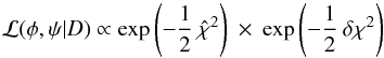$\mathrm{ℒ}\mathrm{\left(}\mathit{\phi ,\psi }\mathrm{\right|}\mathit{D}\mathrm{)}\mathrm{\propto }\exp \left(\mathrm{-}\frac{\mathrm{1}}{\mathrm{2}}\mathit{\chi ̂}\mathrm{2}\right)\mathrm{\times }\exp \left(\mathrm{-}\frac{\mathrm{1}}{\mathrm{2}}\mathit{\delta }{\mathit{\chi }}^{\mathrm{2}}\right)$(9)where is the minimum value of χ² at fixed φ, and δχ²(δψ | φ) is the positive increment in χ² for the displacement . The second factor in Eq. (9) can be eliminated using Eq. (A.9), so that 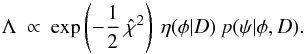$\mathrm{\Lambda }\mathrm{\propto }\exp \left(\mathrm{-}\frac{\mathrm{1}}{\mathrm{2}}\mathit{\chi ̂}\mathrm{2}\right)\mathit{\eta }\mathrm{\left(}\mathit{\phi }\mathrm{\right|}\mathit{D}\mathrm{\left)}\mathit{p}\mathrm{\right(}\mathit{\psi }\mathrm{\left|}\mathit{\phi ,D}\mathrm{\right)}\mathit{.}$(10)If we now approximate p(ψ | φ,D) by a sum of δ functions as discussed in Sect. A.3, then 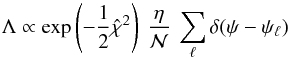$\mathrm{\Lambda }\mathrm{\propto }\exp \left(\mathrm{-}\frac{\mathrm{1}}{\mathrm{2}}\mathit{\chi ̂}\mathrm{2}\right)\frac{\mathit{\eta }}{\mathrm{𝒩}}\sum _{\mathit{\ell }}\mathit{\delta }\mathrm{(}\mathit{\psi }\mathrm{-}{\mathit{\psi }}_{\mathit{\ell }}\mathrm{)}$(11)where the ψ_ℓ are independent vectors that randomly sample the exact quadrivariate normal PDF.

The PDF Λ is for the Thiele-Innes elements. The corresponding PDF Γ(θ | D) for the Campbell elements θ is 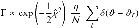$\mathrm{\Gamma }\mathrm{\propto }\exp \left(\mathrm{-}\frac{\mathrm{1}}{\mathrm{2}}\mathit{\chi ̂}\mathrm{2}\right)\frac{\mathit{\eta }}{\mathrm{𝒩}}\sum _{\mathit{\ell }}\mathit{\delta }\mathrm{(}\mathit{\vartheta }\mathrm{-}{\mathit{\vartheta }}_{\mathit{\ell }}\mathrm{)}$(12)where ϑ_ℓ = ϑ(ψ_ℓ).

4.2. Credibility intervals

In terms of a 3D scan over φ-space, the PDF Γ(θ | D) is approximated by the ensemble of 7D vectors ${\mathit{\theta }}_{\mathit{m}}\mathrm{=}\mathrm{\left(}{\mathit{\phi }}_{\mathit{ijk}}\mathit{,}{\mathit{\vartheta }}_{\mathit{\ell }}\mathrm{\right)}$(13)with weights ${\mathit{\mu }}_{\mathit{m}}\mathrm{=}\frac{{\mathit{\eta }}_{\mathit{ijk}}}{\mathrm{𝒩}}\exp \left(\mathrm{-}\frac{\mathrm{1}}{\mathrm{2}}\mathit{\chi ̂}\begin{array}{c}\mathrm{2}\\ \mathit{ijk}\end{array}\right)$(14)Here m is an index that enumerates the random points ϑ_ℓ across all grid points (i,j,k).

If Q(θ) is a quantity for which a credibility interval is required, the data from which this can be computed are the values Q_m = Q(θ_m) with weights μ_m. From this data, an estimate of the PDF of Q is $\mathrm{\Theta }\mathrm{\left(}\mathit{Q}\mathrm{\right)}\mathrm{=}\sum _{\mathit{m}}{\mathit{\mu }}_{\mathit{m}}\mathit{\delta }\mathrm{(}\mathit{Q}\mathrm{-}{\mathit{Q}}_{\mathit{m}}\mathrm{)}\mathit{/}\sum _{\mathit{m}}\mathit{\mu }m$(15)with corresponding cumulative distribution function (CDF) $\mathit{F}\mathrm{\left(}\mathit{Q}\mathrm{\right)}\mathrm{=}\sum _{{\mathit{Q}}_{\mathit{m}}\mathit{<}\mathit{Q}}{\mathit{\mu }}_{\mathit{m}}\mathit{/}\sum _{\mathit{m}}{\mathit{\mu }}_{\mathit{m}}\mathit{.}$(16)The equal tail credibility interval (Q_L,Q_U) corresponding to ± 1σ is then obtained from the equations $\mathit{F}\mathrm{\left(}{\mathit{Q}}_{\mathit{L}}\mathrm{\right)}\mathrm{=}\mathrm{0.1587}\mathit{F}\mathrm{\left(}{\mathit{Q}}_{\mathit{U}}\mathrm{\right)}\mathrm{=}\mathrm{0.8413}$(17)so that the enclosed probability 0.6826.

These credibility intervals are asymptotically rigorous – i.e., are exact in the limits and grid steps → 0.

4.3. Calculation procedure

The basic steps required to derive credibility intervals are as follows:

• 1)

  At every point (log P_i,e_j,τ_k), the minimum-χ² Thiele-Innes elements are obtained with Eqs. (A.7) of L14, and the corresponding $\mathit{\chi ̂}\begin{array}{c}\mathrm{2}\\ \mathit{ijk}\end{array}$ computed.

• 2)

  The variances and covariances defining the exact quadrivariate normal PDF p(ψ | φ,D) at φ_ijk are computed with Eqs. (A.9), (A.10) of L14.

• 3)

  Random points ψ_ℓ sampling the exact PDF p(ψ | φ_ijk,D) are computed as described in Sect. A.4.

• 4)

  The Campbell elements ϑ_ℓ corresponding to ψ_ℓ are computed as described in Sect. A.4 of L14.

• 5)

  The vectors θ_m are then (φ_ijk,ϑ_ℓ) with weights μ_m given by Eq. (14).

• 6)

  Lastly, credibility intervals are derived from Q_m with the approximate CDF given in Eq. (16).

4.4. An example

To illustrate this procedure, credibility intervals are computed for the orbit $\mathrm{\left(}\begin{array}{c}{}_{\mathrm{˜}}\\ {\mathit{x}}_{\mathit{n}}\end{array}\mathit{,}\begin{array}{c}{}_{\mathrm{˜}}\\ {\mathit{y}}_{\mathit{n}}\end{array}\mathrm{\right)}$ discussed in Sect. 3.4. A scatter diagram analogous to Figs. 1 and 2 is not readily constructed because the points θ_m are not of equal weight. Instead, the confidence intervals derived as in Fig. 2 (but now with ) are compared with the credibility intervals derived from Eqs. (17).

The Δ_ν,α = 1 confidence interval for log a is (− 0.020, 0.006), whereas the equal-tail 68.3% credibility interval is (− 0.019, 0.008). The corresponding intervals for i are and , respectively.

In these calculations, for ${\mathit{\chi }}_{\mathit{ijk}}^{\mathrm{2}}\mathit{<}{\mathit{\chi }}_{\min }^{\mathrm{2}}\mathrm{+}\mathrm{21.85}$ and =1 otherwise. The domain defined by this inequality corresponds to Δ_ν,α with α = 0.9973 and ν = 7, thus ensuring an accurate treatment of the wings of the posterior PDF’s to beyond ± 2σ. Convergence experiments indicate that sufficient accuracy is achieved with .

In contrast to confidence intervals derived from scatter plots such as Fig. 2, the credibility intervals calculated from Eqs. (17) are not biased. Convergence to the asymptote is therefore faster and sufficient accuracy is achieved with a smaller .

4.5. Coverage fractions

For comparison with Sect. 3.5 above and with Sect. 5.5 of L14, coverage fractions for credibility intervals are computed for 10 000 independent realizations of the observed orbit, and an interval is again counted as a success if Q_L<Q_exact<Q_U. The results of this experiment (iii) are given in Table 2.

Because these are credibility not frequentist intervals, there is no rigorous asymptotic expectation that the frequentist fractions should be recovered. Nevertheless, these ideal fractions are closely matched and so the credibility intervals calculated according to Sect. 4.2 can be described as well-calibrated (Drawid 1982).

When Table 2 is compared to Table 1 in L14, we see that the previous low coverage fractions for the ψ-elements log a,i,ω,Ω and for the derived quantity log ℳ are now replaced by fractions close to their frequentist values. This confirms the conjecture in L14 that the shortfall was due to the profile likelihood.

As in Sect. 3.5, statistical rigour is achieved with only a modest increase in the computional burden. Experiment iii required 22% more computer time than experiment i.

When Bayesian estimates depend on informative priors, the PDF π(θ) may have a significant gradient at θ_∗, the elements of a particular binary. A coverage experiment restricted to θ_∗ will then (correctly) deviate from the frequentist expectation. In coverage tests for such cases, each independent orbit $\begin{array}{c}{}_{\mathrm{˜}}\\ {\mathit{x}}_{\mathit{n}}\end{array}\mathit{,}\begin{array}{c}{}_{\mathrm{˜}}\\ {\mathit{y}}_{\mathit{n}}\end{array}$ should also be for a random θ drawn from π(θ).

5. Comparison of estimates

The relative performance of minimum-χ² and Bayesian estimation in experiments ii and iii is summarized in Table 3. The means ⟨ δQ ⟩ and standard deviations s_δQ of the residuals δQ = Q_est − Q_exact are tabulated, where Q_est is either the minimum-χ² value of Q or its posterior mean, and Q_exact is given in Eq. (1).

Table 2 shows that in this test the two estimation methodologies yield closely similiar results. This is to be expected for a non-informative prior π(θ) with negligible gradient at θ_∗.

6. Conclusion

This paper has addressed a technical issue in the statistical analysis of orbits: how to achieve statistical rigour while taking advantage of the linearity of a subset of the orbital elements. The coverage experiments reported in Sects. 3.5 and 4.5 demonstrate that statistical rigour is achieved for both minimum-χ² and Bayesian estimation. Moreover, the reported timings show an inconsequential increase in the computational burden.

The key to this success is that at each grid point the distribution of probability in Thiele-Innes space is known. For minimum-χ² estimation, this allows Monte Carlo sampling to be targeted (Sect. A.5) precisely on the constant χ² surface defining the desired confidence level. For Bayesian estimation, the known PDF allows Monte Carlo sampling in Thiele-Innes space to be concentrated (Sect. A.4) on the high probability domain enclosing the least-squares points . Moreover, in each case, the random sampling does not require additional orbits to be computed.

The approach developed here is not specific to visual binaries or to the Thiele-Innes elements. In principle, an analogous procedure can be constructed for any partially linear estimation problem.

Online material

Appendix A: Statistics in Thiele-Innes space

In Appendix A of L14, formulae are derived for , the least squares Thiele-Innes constants at given φ = (log P,e,τ). The resulting value of χ² then determines the profile likelihood ℒ^† used in the approximation of posterior means – Eq. (7) of L14. Now we wish to sample points displaced from . Let such a displacement be δψ = (a,b,f,g).

Appendix A.1: Probability density function p(ψ | φ, D)

In Sect. A.4 of L14, the PDF at δψ is shown to be the product of two independent PDF’s, each a bivariate normal distribution, one for (a,f), the other for (b,g). Formulae for the variances ${\mathit{\sigma }}_{\mathit{a}}^{\mathrm{2}}\mathit{,}{\mathit{\sigma }}_{\mathit{b}}^{\mathrm{2}}\mathit{,}{\mathit{\sigma }}_{\mathit{f}}^{\mathrm{2}}\mathit{,}{\mathit{\sigma }}_{\mathit{g}}^{\mathrm{2}}$ and the covariances cov(a,f),cov(b,g) that define these PDF’s are given in Eqs. (A.9) and (A.10) of L14.

The PDF for (a,f) is 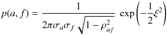$\mathit{p}\mathrm{\left(}\mathit{a,f}\mathrm{\right)}\mathrm{=}\frac{\mathrm{1}}{\mathrm{2}\mathit{\pi }{\mathit{\sigma }}_{\mathit{a}}{\mathit{\sigma }}_{\mathit{f}}\sqrt{\mathrm{1}\mathrm{-}{\mathit{\rho }}_{\mathit{af}}^{\mathrm{2}}}}\exp \left(\mathrm{-}\frac{\mathrm{1}}{\mathrm{2}}{\mathit{\xi }}^{\mathrm{2}}\right)$(A.1)where ρ_af = cov(a,f)/(σ_aσ_f) and ${\mathit{\xi }}^{\mathrm{2}}\mathrm{=}\frac{\mathrm{1}}{\mathrm{1}\mathrm{-}{\mathit{\rho }}_{\mathit{af}}^{\mathrm{2}}}\left[{\left(\frac{\mathit{a}}{{\mathit{\sigma }}_{\mathit{a}}}\right)}^{\mathrm{2}}\mathrm{+}{\left(\frac{\mathit{f}}{{\mathit{\sigma }}_{\mathit{f}}}\right)}^{\mathrm{2}}\mathrm{-}\mathrm{2}{\mathit{\rho }}_{\mathit{af}}\left(\frac{\mathit{a}}{{\mathit{\sigma }}_{\mathit{a}}}\right)\left(\frac{\mathit{f}}{{\mathit{\sigma }}_{\mathit{f}}}\right)\right]$(A.2)The point (0,0) corresponds to the minimum-${\mathit{\chi }}_{\mathit{x}}^{\mathrm{2}}$ solution , where ${\mathit{\chi }}_{\mathit{x}}^{\mathrm{2}}$ is the x-coordinate contribution to χ² – see Eq. (2). The displacement (a,f) therefore results in a positive increment $\mathit{\delta }{\mathit{\chi }}_{\mathit{x}}^{\mathrm{2}}$ given by ${\mathit{\sigma }}^{\mathrm{2}}\mathit{\delta }{\mathit{\chi }}_{\mathit{x}}^{\mathrm{2}}\mathrm{=}{\mathrm{\Sigma }}_{\mathit{n}}{\mathit{w}}_{\mathit{n}}\mathrm{\left[}\mathrm{\right(}{\mathit{x}}_{\mathit{n}}\mathrm{-}\begin{array}{c}\mathrm{˜}\\ {\mathit{x}}_{\mathit{n}}\end{array}{\mathrm{)}}^{\mathrm{2}}\mathrm{-}\mathrm{(}\mathit{x̂}\mathit{n}\mathrm{-}\begin{array}{c}\mathrm{˜}\\ {\mathit{x}}_{\mathit{n}}\end{array}{\mathrm{)}}^{\mathrm{2}}\mathrm{]}\mathit{.}$(A.3)Now, for displacement (a,f), the predicted ${\mathit{x}}_{\mathit{n}}\mathrm{=}\mathit{x̂}\mathit{n}\mathrm{+}\mathit{a}{\mathit{X}}_{\mathit{n}}\mathrm{+}\mathit{fY}n$(A.4)where X,Y are given by Eqs. (A.3) in L14. Substitution in Eq. (A.3) then gives ${\mathit{\sigma }}^{\mathrm{2}}\mathit{\delta }{\mathit{\chi }}_{\mathit{x}}^{\mathrm{2}}\mathrm{=}{\mathrm{\Sigma }}_{\mathit{n}}{\mathit{w}}_{\mathit{n}}\mathrm{(}{\mathit{a}}^{\mathrm{2}}{\mathit{X}}_{\mathit{n}}^{\mathrm{2}}\mathrm{+}{\mathit{f}}^{\mathrm{2}}{\mathit{Y}}_{\mathit{n}}^{\mathrm{2}}\mathrm{+}\mathrm{2}\mathit{af}{\mathit{X}}_{\mathit{n}}{\mathit{Y}}_{\mathit{n}}\mathrm{)}$(A.5)where terms linear in a and f vanish because the minimum is at (0,0). The summations in Eq. (A.5) can be eliminated in favour of ${\mathit{\sigma }}_{\mathit{a}}^{\mathrm{2}}\mathit{,}{\mathit{\sigma }}_{\mathit{f}}^{\mathrm{2}}$ and cov(a,f) with the formulae given in Eqs. (A.6), (A.9) and (A.10) of L14. After lengthy algebra, we find that $\mathit{\delta }{\mathit{\chi }}_{\mathit{x}}^{\mathrm{2}}\mathrm{=}\frac{\mathrm{1}}{\mathrm{1}\mathrm{-}{\mathit{\rho }}_{\mathit{af}}^{\mathrm{2}}}\left[{\left(\frac{\mathit{a}}{{\mathit{\sigma }}_{\mathit{a}}}\right)}^{\mathrm{2}}\mathrm{+}{\left(\frac{\mathit{f}}{{\mathit{\sigma }}_{\mathit{f}}}\right)}^{\mathrm{2}}\mathrm{-}\mathrm{2}{\mathit{\rho }}_{\mathit{af}}\left(\frac{\mathit{a}}{{\mathit{\sigma }}_{\mathit{a}}}\right)\left(\frac{\mathit{f}}{{\mathit{\sigma }}_{\mathit{f}}}\right)\right]$(A.6)and so $\mathit{p}\mathrm{\left(}\mathit{a,f}\mathrm{\right)}\mathrm{\propto }\exp \left(\mathrm{-}\frac{\mathrm{1}}{\mathrm{2}}\mathit{\delta }{\mathit{\chi }}_{\mathit{x}}^{\mathrm{2}}\right)\mathit{.}$(A.7)Exactly the same analysis applies to the independent pair (b,g), so that $\mathit{p}\mathrm{\left(}\mathit{b,g}\mathrm{\right)}\mathrm{\propto }\exp \left(\mathrm{-}\frac{\mathrm{1}}{\mathrm{2}}\mathit{\delta }{\mathit{\chi }}_{\mathit{y}}^{\mathrm{2}}\right)\mathit{.}$(A.8)Combining these formulae, we find that the PDF at is $\mathit{p}\mathrm{\left(}\mathit{\psi }\mathrm{\right|}\mathit{\phi ,D}\mathrm{)}\mathrm{=}\frac{\mathrm{1}}{\mathrm{4}{\mathit{\pi }}^{\mathrm{2}}{\mathit{\sigma }}^{\mathrm{4}}\mathit{\eta }}\exp \left(\mathrm{-}\frac{\mathrm{1}}{\mathrm{2}}\mathit{\delta }{\mathit{\chi }}^{\mathrm{2}}\right)$(A.9)where $\mathit{\delta }{\mathit{\chi }}^{\mathrm{2}}\mathrm{=}\mathit{\delta }{\mathit{\chi }}_{\mathit{x}}^{\mathrm{2}}\mathrm{+}\mathit{\delta }{\mathit{\chi }}_{\mathit{y}}^{\mathrm{2}}$ and η(φ | D) is given by ${\mathit{\sigma }}^{\mathrm{4}}\mathit{\eta }\mathrm{=}{\mathit{\sigma }}_{\mathit{a}}{\mathit{\sigma }}_{\mathit{f}}\sqrt{\mathrm{(}}\mathrm{1}\mathrm{-}{\mathit{\rho }}_{\mathit{af}}^{\mathrm{2}}\mathrm{)}\mathrm{\times }{\mathit{\sigma }}_{\mathit{b}}{\mathit{\sigma }}_{\mathit{g}}\sqrt{\mathrm{(}}\mathrm{1}\mathrm{-}{\mathit{\rho }}_{\mathit{bg}}^{\mathrm{2}}\mathrm{)}$(A.10)

Appendix A.2: Modified Thiele-Innes constants

The familiar device of “completing the square” applied to Eq. (A.2) suggests new variables defined by $\frac{\mathit{a}}{{\mathit{\sigma }}_{\mathit{a}}}\mathrm{=}\mathrm{𝒜}\mathit{,}\frac{\mathit{f}}{{\mathit{\sigma }}_{\mathit{f}}}\mathrm{=}{\mathit{\rho }}_{\mathit{af}}\mathrm{𝒜}\mathrm{+}\sqrt{\mathrm{1}\mathrm{-}{\mathit{\rho }}_{\mathit{af}}^{\mathrm{2}}}\mathrm{ℱ}\mathit{.}$(A.11)Substitution in Eq. (A.6) then gives $\mathit{\delta }{\mathit{\chi }}_{\mathit{x}}^{\mathrm{2}}\mathrm{=}{\mathrm{𝒜}}^{\mathrm{2}}\mathrm{+}{\mathrm{ℱ}}^{\mathrm{2}}\mathit{.}$(A.12)The Jacobian of this transformation is $\frac{\mathit{\partial }\mathrm{\left(}\mathit{a,f}\mathrm{\right)}}{\mathit{\partial }\mathrm{\left(}\mathrm{𝒜}\mathit{,}\mathrm{ℱ}\mathrm{\right)}}\mathrm{=}{\mathit{\sigma }}_{\mathit{a}}{\mathit{\sigma }}_{\mathit{f}}\sqrt{\mathrm{1}\mathrm{-}{\mathit{\rho }}_{\mathit{af}}^{\mathrm{2}}}$(A.13)so that, by conservation of probability, the PDF of is $\mathrm{\Psi }\mathrm{\left(}\mathrm{𝒜}\mathit{,}\mathrm{ℱ}\mathrm{\right)}\mathrm{=}\frac{\mathrm{1}}{\mathrm{2}\mathit{\pi }}\exp \left[\mathrm{-}\frac{\mathrm{1}}{\mathrm{2}}\mathrm{(}{\mathrm{𝒜}}^{\mathrm{2}}\mathrm{+}{\mathrm{ℱ}}^{\mathrm{2}}\mathrm{)}\right]\mathit{.}$(A.14)Now, exactly the same analysis applies to the independent pair (b,g). Thus, if we define new variables by the equations $\begin{array}{ccc}\frac{\mathit{b}}{{\mathit{\sigma }}_{\mathit{b}}}\mathrm{=}\mathrm{ℬ}\mathit{,}\frac{\mathit{g}}{{\mathit{\sigma }}_{\mathit{g}}}\mathrm{=}{\mathit{\rho }}_{\mathit{bg}}\mathrm{ℬ}\mathrm{+}\sqrt{\mathrm{1}\mathrm{-}{\mathit{\rho }}_{\mathit{bg}}^{\mathrm{2}}}& & \end{array}$(A.15)then the PDF of is , and $\mathit{\delta }{\mathit{\chi }}_{\mathit{y}}^{\mathrm{2}}\mathrm{=}{\mathrm{ℬ}}^{\mathrm{2}}\mathrm{+}{\mathrm{𝒢}}^{\mathrm{2}}\mathit{.}$(A.16)If ζ denotes the vector , then Π(ζ), the PDF in ζ-space, is – i.e., $\mathrm{\Pi }\mathrm{\left(}\mathit{\zeta }\mathrm{\right)}\mathrm{=}\frac{\mathrm{1}}{\mathrm{4}{\mathit{\pi }}^{\mathrm{2}}}\exp \left[\mathrm{-}\frac{\mathrm{1}}{\mathrm{2}}\mathrm{(}{\mathrm{𝒜}}^{\mathrm{2}}\mathrm{+}{\mathrm{ℬ}}^{\mathrm{2}}\mathrm{+}{\mathrm{ℱ}}^{\mathrm{2}}\mathrm{+}{\mathrm{𝒢}}^{\mathrm{2}}\mathrm{)}\right]\mathit{.}$(A.17)Accordingly, the distribution of probability in ζ-space is simply the product of four independent normal distributions, each with zero mean and unit variance.

The increment in χ² is given by Eqs. (A.12) and (A.16) as $\mathit{\delta }{\mathit{\chi }}^{\mathrm{2}}\mathrm{\left(}\mathit{\zeta }\mathrm{\right)}\mathrm{=}{\mathrm{𝒜}}^{\mathrm{2}}\mathrm{+}{\mathrm{ℬ}}^{\mathrm{2}}\mathrm{+}{\mathrm{ℱ}}^{\mathrm{2}}\mathrm{+}{\mathrm{𝒢}}^{\mathrm{2}}\mathit{.}$(A.18)

Appendix A.3: Approximate PDFs

A distribution of probability can be represented by a sum of δ functions in such a way that the probability attached to any finite element of space is approximated with arbitrary accuracy. Thus, the PDF giving the distribution of probability in ζ-space is given approximately by $\mathit{p}\mathrm{\left(}\mathit{\zeta }\mathrm{\right)}\mathrm{=}{\mathrm{𝒩}}^{-1}\sum _{\mathit{\ell }}\mathit{\delta }\mathrm{(}\mathit{\zeta }\mathrm{-}{\mathit{\zeta }}_{\mathit{\ell }}\mathrm{)}$(A.19)where each ζ_ℓ is an independent random vector sampling the PDF Π(ζ) given by Eq. (A.17). The integral of p(ζ) over a finite element in ζ-space converges to the exact value as .

Equations (A.11) and (A.15) transform the point ζ_ℓ into the displacement . The corresponding approximate PDF in ψ-space is therefore $\mathit{p}\mathrm{\left(}\mathit{\psi }\mathrm{\right|}\mathit{\phi ,D}\mathrm{)}\mathrm{=}{\mathrm{𝒩}}^{-1}\sum _{\mathit{\ell }}\mathit{\delta }\mathrm{(}\mathit{\psi }\mathrm{-}{\mathit{\psi }}_{\mathit{\ell }}\mathrm{)}\mathit{.}$(A.20)Note that the Jacobian of this transformation from ζ- to ψ- space is implicit in the changes in number densities of the delta functions in the respective spaces.

Similarly, the PDF for the Campbell elements ϑ corresponding to the Thiele-Innes elements ψ is $\mathit{p}\mathrm{\left(}\mathit{\vartheta }\mathrm{\right|}\mathit{\phi ,D}\mathrm{)}\mathrm{=}{\mathrm{𝒩}}^{-1}\sum _{\mathit{\ell }}\mathit{\delta }\mathrm{(}\mathit{\vartheta }\mathrm{-}{\mathit{\vartheta }}_{\mathit{\ell }}\mathrm{)}$(A.21)where ϑ_ℓ = ϑ(ψ_ℓ) is derived as described in Sect. A.4 of L14.

Appendix A.4: Random sampling in ψ-space

According to Eq. (A.17), a random point in ζ-space is (z₁,z₂,z₃,z₄), where the z_i are independent random Gaussian variates drawn from . This point corresponds to the displacement (a,b,f,g) given by Eqs. (A.11) and (A.15) and therefore to the point in ψ-space. Thus, a point randomly selected from the exact PDF p(ψ | φ,D) can be derived from four independent Gaussian variates, and the resulting increment in χ² is given by Eq. (A.18) as $\mathit{\delta }{\mathit{\chi }}^{\mathrm{2}}\mathrm{\left(}\mathit{\psi }\mathrm{\right)}\mathrm{=}{\mathit{z}}_{\mathrm{1}}^{\mathrm{2}}\mathrm{+}{\mathit{z}}_{\mathrm{2}}^{\mathrm{2}}\mathrm{+}{\mathit{z}}_{\mathrm{3}}^{\mathrm{2}}\mathrm{+}{\mathit{z}}_{\mathrm{4}}^{\mathrm{2}}$(A.22)

Appendix A.5: Random sampling at fixed δχ²

A random point in ψ-space subject to a constraint on δχ² can be found by first selecting a random point on the 4D sphere in ζ-space defined by Eq. (A.18). This is achieved as follows: If z_i again denotes a Gaussian variate from , then a random point on this hypersphere is (z₁,z₂,z₃,z₄) /Z, where ${\mathit{Z}}^{\mathrm{2}}\mathrm{=}\mathrm{(}{\mathit{z}}_{\mathrm{1}}^{\mathrm{2}}\mathrm{+}{\mathit{z}}_{\mathrm{2}}^{\mathrm{2}}\mathrm{+}{\mathit{z}}_{\mathrm{3}}^{\mathrm{2}}\mathrm{+}{{\mathit{z}}_{\mathrm{4}}^{\mathrm{2}}}^{\mathrm{)}}\mathit{/}\mathit{\delta \chi }2$(A.23)(Muller 1979). The corresponding point (A,B,F,G) in ψ-space is then derived from Eqs. (A.11) and (A.15).

The random sampling procedures of Sects. A.4 and A.5 predict χ² without the need to compute an orbit. This is achieved by exploiting the linearity of the ψ-elements and is the basis of the computational efficiency of the techniques of Sects. 3.3 and 4.1. However, during code development, this prediction should be tested by actually computing the orbit and independently evaluating χ² from Eq. (2).

Acknowledgments

The issue of error underestimation in hybrid problems was raised by the referee of the previous paper (L14) and was the direct stimulus of this investigation. This same referee provided useful comments on this paper.

References

All Tables

All Figures

	Fig. 1 Approximate confidence intervals. The ensemble of orbit vectors with $\mathit{\chi ̂}\begin{array}{c}\mathrm{2}\\ \mathit{ijk}\end{array}\mathit{<}{\mathit{\chi }}_{\min }^{\mathrm{2}}\mathrm{+}\mathrm{1}$ is projected on to the (log a,i)-plane. The ± 1σ bounds for each coordinate are indicated. The 506 grid points φijk define the domain .
In the text

	Fig. 2 Accurate confidence limits. The ensemble of orbit vectors – i.e., with ${\mathit{\chi }}_{\mathit{\ell }}^{\mathrm{2}}\mathrm{=}{\mathit{\chi }}_{\min }^{\mathrm{2}}\mathrm{+}\mathrm{1}$ – is projected on to the (log a,i)-plane. The ± 1σ bounds for each coordinate are indicated. Each of the 506 grid points gives rise to points on .
In the text

References

- Dawid, A. P. 1982, J. Am. Stat. Assoc., 77, 605 [CrossRef] [Google Scholar]
- Eastman, J., Gaudi, B., & Agol, E. 2013, PASP, 125, 83 [NASA ADS] [CrossRef] [Google Scholar]
- Hartkopf, W. I., McAlister, H. A., & Franz, O. G. 1989, AJ, 98, 1014 [NASA ADS] [CrossRef] [Google Scholar]
- James, F. 2006, Statistical Methods in Experimental Physics (Singapore: World Scientific Publishing Co.) [Google Scholar]
- Lucy, L. B. 2014, A&A, 563, 126 (L14) [Google Scholar]
- Muller, M. E. 1959, Comm. Assoc. Comp. Mach., 2, 19 [Google Scholar]
- Press, W. H., Teukolsky, S. A., Vetterling, W. T., & Flannery, B. P. 1992, Numerical Recipes, 2nd edn. (Cambridge: Cambridge Univ. Press) [Google Scholar]
- Schaefer, G. H., Simon, M., Beck, T. L., Nelan, E., & Prato, L. 2006, AJ, 132, 2618 [NASA ADS] [CrossRef] [Google Scholar]