| Issue |
A&A
Volume 565, May 2014
|
|
|---|---|---|
| Article Number | A78 | |
| Number of page(s) | 4 | |
| Section | The Sun | |
| DOI | https://doi.org/10.1051/0004-6361/201423536 | |
| Published online | 14 May 2014 | |
Research Note
Determination of the cross-field density structuring in coronal waveguides using the damping of transverse waves
1
Instituto de Astrofísica de Canarias,
38205
La Laguna, Tenerife
Spain
e-mail: This email address is being protected from spambots. You need JavaScript enabled to view it.
2
Departamento de Astrofísica, Universidad de La
Laguna, 38206, La
Laguna, Tenerife,
Spain
Received:
29
January
2014
Accepted:
2
April
2014
Abstract
Context. Time and spatial damping of transverse magnetohydrodynamic (MHD) kink oscillations is a source of information on the cross-field variation of the plasma density in coronal waveguides.
Aims. We show that a probabilistic approach to the problem of determining the density structuring from the observed damping of transverse oscillations enables us to obtain information on the two parameters that characterise the cross-field density profile.
Methods. The inference is performed by computing the marginal posterior distributions for density contrast and transverse inhomogeneity length-scale using Bayesian analysis and damping ratios for transverse oscillations under the assumption that damping is produced by resonant absorption.
Results. The obtained distributions show that, for damping times of a few oscillatory periods, low density-contrasts and short inhomogeneity length scales are more plausible to explain observations.
Conclusions. This means that valuable information on the cross-field density profile can be obtained even if the inversion problem, with two unknowns and one observable, is a mathematically ill-posed problem.
Key words: magnetohydrodynamics (MHD) / waves / methods: statistical / Sun: corona / Sun: oscillations
© ESO, 2014
1. Introduction
Transverse magnetohydrodynamic (MHD) kink oscillations have been reported in numerous observations of solar coronal magnetic and plasma structures. First revealed in coronal loop observations using the Transition Region And Coronal Explorer (TRACE) by Aschwanden et al. (1999) and Nakariakov et al. (1999), they also seem to be an important part of the dynamics of chromospheric spicules and mottles (De Pontieu et al. 2007; Kuridze et al. 2013); soft X-ray coronal jets (Cirtain et al. 2007); or prominence fine structures (Okamoto et al. 2007; Lin et al. 2009). Their presence over extended regions of the solar corona (Tomczyk et al. 2007) may have implications on the role of waves in coronal heating. Observations with instruments such as AIA/SDO, CoMP, and Hi-C by e.g. Morton & McLaughlin (2013) and Threlfall et al. (2013) have allowed us to analyse transverse oscillations in unprecedented detail.
The potential use of transverse oscillations as a diagnostic tool to infer otherwise difficult-to-measure coronal magnetic and plasma properties was first demonstrated by Nakariakov & Ofman (2001) by interpreting them as MHD kink modes of magnetic flux tubes. Since then, a number of studies have used seismology diagnostic tools that make use of oscillation properties, such as periods and damping times, to obtain information on the magnetic field and plasma density structuring (see e.g. Andries et al. 2005; Arregui et al. 2007; Verth et al. 2008, 2011). An overview of recent seismology applications can be found in Arregui (2012) and De Moortel & Nakariakov (2012). The increase in the number of observed events has lately enabled the application of statistical techniques to seismology diagnostics (Verwichte et al. 2013; Asensio Ramos & Arregui 2013).
Some of these studies are concerned with the determination of the cross-field density structuring in waveguides supporting MHD oscillations. Goossens et al. (2002) were the first to note that measurements of the damping rate of coronal loop oscillations together with the assumption of resonant absorption as the damping mechanism could be used to obtain estimates for the transverse inhomogeneity length scale. By assuming a value for the ratio of the plasma density between the interior of the loop and the corona, they computed the inhomogeneity length scale for a set of 11 loop oscillation events. Verwichte et al. (2006) analysed how information on the density profile across arcade-shaped models can be obtained from the oscillation properties of vertically polarised transverse waves. When no assumption is made on the density contrast, Arregui et al. (2007) and Goossens et al. (2008) showed that an infinite number of equally valid equilibrium models is able to reproduce observed damping rates, although they must follow a particular one-dimensional curve in the two-dimensional parameter space of unknowns. More recently, Arregui & Asensio Ramos (2011) have shown how information on density contrast from observations can be used as prior information in order to fully constrain the transverse density structuring of coronal loops. Arregui et al. (2013) have shown that the existence of two regimes in the damping time/spatial scales would enable the constraint of both the density contrast and its transverse inhomogeneity length scale. The feasibility of such a measurement has yet to be confirmed by observations.
We present the Bayesian solution to the problem, which makes use of the computation of marginal posteriors, and show that valuable information on the cross-field density profile can be obtained even if the inversion problem, with two unknowns and one observable, is a mathematically ill-posed problem.
2. Conditional probability and marginal posteriors
Consider the determination of a set of parameters θ related to a
theoretical model, M, that are compared to observed data, d. Bayes’ rule for
conditional probability (Bayes & Price 1763)
states that the probability of θ taking on given values, conditional
on the observed data, i.e. the posterior probability p(θ|d), is a combination of how well the data are
reproduced by the model parameters, i.e. the likelihood function p(d|θ), and the probability of the
parameters independent of the data, i.e. the prior distribution p(θ). These quantities
are related as follows  (1)and we have made explicit
that all quantities are conditional on the assumed model M. The denominator is the
so-called evidence, an integral of the likelihood over the prior distribution that
normalises the likelihood and turns it into a probability. The prior and likelihood
represent probabilities that are directly assigned, whilst the posterior is computed.
Probability in this context means the grade of belief in a statement about the value a
parameter can take on, conditional on observed data. The resulting posterior is a
distribution that quantifies this grade of belief.
(1)and we have made explicit
that all quantities are conditional on the assumed model M. The denominator is the
so-called evidence, an integral of the likelihood over the prior distribution that
normalises the likelihood and turns it into a probability. The prior and likelihood
represent probabilities that are directly assigned, whilst the posterior is computed.
Probability in this context means the grade of belief in a statement about the value a
parameter can take on, conditional on observed data. The resulting posterior is a
distribution that quantifies this grade of belief.
Once the full posterior is known, the so-called marginal posterior enables us to calculate
how a particular parameter of interest, θi, is constrained by
observations, by just performing an integral of the posterior over the rest of the model
parameters:  (2)This quantity
encodes all information for model parameter θi available in the
priors and the data and correctly propagates uncertainty in the rest of the parameters to
the one of interest.
(2)This quantity
encodes all information for model parameter θi available in the
priors and the data and correctly propagates uncertainty in the rest of the parameters to
the one of interest.
Consider an observable quantity, c, which, according to some theoretical model with parameters a and b is predicted to be related to them by a given forward model, cmodel = f(a,b), indicating that c is a function of a and b. A given value of c can be obtained from different combinations of a and b. The observational measurement of c provides us with many equally valid combinations of a and b that give the observed c. In a real application, measurements are corrupted by noise, which makes a probabilistic approach to the inversion problem necessary.
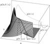 |
Fig. 1 Surface plot of the joint probability p(a,b | c) of parameters a and b for a given observation of c according to the forward model cmodel = a·b and assuming a Gaussian likelihood (Eq. (3)). Conditional probabilities for selected values of parameters are indicated by arrows. Marginal posteriors are projected onto the two vertical planes. |
In our analysis, we consider that observations are corrupted with Gaussian noise and that
they are statistically independent. Then, the observed values of c and the theoretical
predictions can be compared by adopting a Gaussian likelihood of the form ![Mathematical equation: \begin{equation} \label{like1} p(c|a,b) = \frac{1}{\sqrt{2\pi}\sigma_c} \exp \left\{-\frac{\left[c-c_{\mathrm{model}}(a,b)\right]^2}{2 \sigma^2_c} \right\}, \end{equation}](/articles/aa/full_html/2014/05/aa23536-14/aa23536-14-eq16.png) (3)with σc the uncertainty
associated to the measured c. We also assume uniform prior distributions for
a and
b over given
ranges that are irrelevant to our current discussion. The actual capability of the model to
reproduce the observation can be evaluated by computing the joint probability of
a and
b,
conditional on c. Figure 1
displays this two-dimensional distribution where the forward model is simply the product of
a and
b. This
forward model is chosen here for simplicity. Any other choice is equally valid to describe
our approach. At each position, the magnitude of the joint probability p(a,b|c) inform us on the ability of that particular
combination of parameters to reproduce a particular value for the observed c.
(3)with σc the uncertainty
associated to the measured c. We also assume uniform prior distributions for
a and
b over given
ranges that are irrelevant to our current discussion. The actual capability of the model to
reproduce the observation can be evaluated by computing the joint probability of
a and
b,
conditional on c. Figure 1
displays this two-dimensional distribution where the forward model is simply the product of
a and
b. This
forward model is chosen here for simplicity. Any other choice is equally valid to describe
our approach. At each position, the magnitude of the joint probability p(a,b|c) inform us on the ability of that particular
combination of parameters to reproduce a particular value for the observed c.
A cut on this surface along the direction of the parameter b, at a particular value of the parameter a, is the probability of b conditional on a and the observation c, p(b|a,c). A cut for another value for a will result in a different probability distribution for b. The full probability of b, conditional only on data is the integral over all possible values for a, i.e. the marginal posterior p(b|c). Correspondingly, a cut along the direction of the parameter a, at a particular value of the parameter b, is the probability of a, conditional on b and c, p(a|b,c). The full probability of a, conditional on data is the integral over all possible values for b, i.e. the marginal posterior p(a|c). The two marginal posteriors for a and b are shown on the vertical planes in Fig. 1. They indicate that even if the observed c can be reproduced by many combinations (product of values) of a and b, some parameter values are more plausible than others. The particular result will depend on the forward model, which determines the shape of the joint distribution, the data value with its associated uncertainty, and the range over which parameters are allowed to vary (the priors).
3. The probability of a damping ratio
As an application of the procedure outlined above, we consider the damping of transverse
MHD kink waves by resonant absorption in one-dimensional density tube models for coronal
waveguides. The classic analysis in the thin tube and thin boundary approximations (Goossens et al. 1992; Ruderman & Roberts 2002) leads to the expression for the damping ratio,
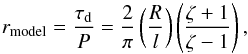 (4)with P and τd the period and
damping time of the oscillation, ζ =
ρi/ρe
the density contrast, and l/R the transverse
inhomogeneity length scale in units of the tube radius R. The factor 2 /π arises
from the assumed sinusoidal variation of the density profile at the tube boundary. The
impact of alternative density profiles on seismology estimates is discussed in Soler et al. (2014). A similar expression is valid for
propagating kink waves upon replacement of the damping time τd by the damping
length Ld and of the oscillation period
P by the
longitudinal wavenumber kz, as shown by Terradas et al. (2010).
(4)with P and τd the period and
damping time of the oscillation, ζ =
ρi/ρe
the density contrast, and l/R the transverse
inhomogeneity length scale in units of the tube radius R. The factor 2 /π arises
from the assumed sinusoidal variation of the density profile at the tube boundary. The
impact of alternative density profiles on seismology estimates is discussed in Soler et al. (2014). A similar expression is valid for
propagating kink waves upon replacement of the damping time τd by the damping
length Ld and of the oscillation period
P by the
longitudinal wavenumber kz, as shown by Terradas et al. (2010).
In our particular application, the two unknown parameters θ =
(ζ,l/R) will be
inferred using the damping ratio as an observable, d = r,
assuming the resonant damping model, M, as the explanation for the decay of the
oscillations. We proceed as in Sect. 2 and assign
direct probabilities for the likelihood function and the prior distribution. We adopt a
Gaussian likelihood function that relates the observed damping ratio, r, and the predictions of the
model, rmodel, given by Eq. (4), so that
![Mathematical equation: \begin{equation} p(r|\zeta, l/R) = \frac{1}{\sqrt{2\pi}\sigma} \exp \left\{-\frac{\left[r-r_{\mathrm{model}}(\zeta, l/R)\right]^2}{2 \sigma^2} \right\}, \end{equation}](/articles/aa/full_html/2014/05/aa23536-14/aa23536-14-eq35.png) (5)with σ the uncertainty associated
to the measured damping ratio. We also adopt uniform prior distributions for both unknowns
over given ranges, so that all the values inside those ranges are equally probable a priori,
so we consider
(5)with σ the uncertainty associated
to the measured damping ratio. We also adopt uniform prior distributions for both unknowns
over given ranges, so that all the values inside those ranges are equally probable a priori,
so we consider  (6)and zero otherwise.
Application of Bayes rule (Eq. (1)) provides
us with the full posterior, p(θ|d), from which the marginal posteriors are obtained
through marginalisation,
(6)and zero otherwise.
Application of Bayes rule (Eq. (1)) provides
us with the full posterior, p(θ|d), from which the marginal posteriors are obtained
through marginalisation,  (7)Figure
2 shows an example inversion result. The inversion
suggests that low density-contrast values are preferred over high contrast ones. However,
the posterior for density contrast displays a long tail, which means that this parameter can
only be constrained with a large uncertainty. A more constrained marginal posterior is
obtained for the transverse inhomogeneity length scale, which points to short values of
l/R to be more
plausible than models with a fully non-uniform layer. The joint two-dimensional distribution
shows the combined posterior distribution for both parameters with the 68% and 95% credible
regions.
(7)Figure
2 shows an example inversion result. The inversion
suggests that low density-contrast values are preferred over high contrast ones. However,
the posterior for density contrast displays a long tail, which means that this parameter can
only be constrained with a large uncertainty. A more constrained marginal posterior is
obtained for the transverse inhomogeneity length scale, which points to short values of
l/R to be more
plausible than models with a fully non-uniform layer. The joint two-dimensional distribution
shows the combined posterior distribution for both parameters with the 68% and 95% credible
regions.
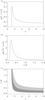 |
Fig. 2 a) and b) Marginal posteriors for ζ and l/R for an inversion with a measured damping ratio r = 3 and σ = 1, using uniform priors in the ranges ζ ∈ [ 1.1−10 ] and l/R ∈ [0.01−2]. c) Joint two-dimensional posterior distribution for the two inferred parameters. The light and dark grey shaded regions indicate the 95% and 68% credible regions, respectively. |
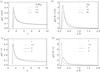 |
Fig. 3 a) and b) Effect of different prior ranges with l/R ∈ [ 0.01,(l/R)max ] on the marginal posterior for ζ and with ζ ∈ [ 1.1,ζmax] on the marginal posterior for l/R. c) and d) Effect of three different damping ratio measurements on the inferred marginal posteriors. In all figures, σ = 1. |
Inferences depend on the assumed prior ranges, since the integrals run over the assumed parameter ranges. The values for ζmin and (l/R)min were chosen so that they are slightly above the minimum values permitted by the theoretical model. Figure 3a shows that varying the upper limit of the transverse inhomogeneity length scale in its prior distribution does not affect the determination of density contrast much. Alternatively, varying the upper limit of the considered density contrast in its prior distribution results in marginal posteriors for l/R that shift towards shorter transverse inhomogeneity length scales being more plausible (Fig. 3b).
Observed damping ratios in e.g. coronal loop oscillations are roughly between 1 and 5. We have performed the inference for three particular values (see Figs. 3c and d). We find that damping ratios slightly larger than one do not enable us to constrain the unknown parameters using this method (dotted lines). Once the damping time is several times the period, e.g. r = 3, well constrained distributions are obtained (solid lines). Finally, larger damping ratios still enable us to constrain l/R, but the only statement that can be made regarding the density contrast is that low values are more plausible than larger ones (dashed lines). In all our computations, with damping times of a few oscillatory periods, short transverse inhomogeneity length scales are always found to be the most plausible ones.
4. Conclusions
Seismology of transverse MHD kink oscillations offers a way to obtain information on the plasma density structuring across magnetic waveguides. For resonantly damped kink mode oscillations, the determination of the cross-field density profile from observed damping ratios consists of the solution of an ill-posed mathematical problem with two unknowns and one observable
In this study we have introduced a modified Bayesian analysis technique that makes use of the basic definition of marginal posteriors, which are obtained not by sampling the posterior using a Markov chain Monte Carlo technique as in Arregui & Asensio Ramos (2011), but by performing the required integrals over the parameter space once the joint probability is computed. This has led to a better understanding of when and how the unknown parameters may be constrained.
The application of this technique for the computation of the probability distribution of the unknowns enables us to draw conclusions about the most plausible values, conditional on observed data. The procedure makes use of all available information and offers correctly propagated uncertainty. Considering typical ranges for the possible values of the unknown parameters we find that, for damping times of a few oscillatory periods, low values for the density contrast are favoured and larger values of this parameter become less plausible. Regarding the transverse inhomogeneity length scale, short values below the scale of the tube radius are found to be more plausible than longer length-scales near the limit for fully non-uniform tubes.
The procedure described here can be followed to obtain the most plausible values for the two unknowns that determine the cross-field density profile in coronal waveguides, upon assuming resonant absorption as the damping mechanism operating in transverse kink waves, and conditional on the observed damping ratios with their associated uncertainty.
In contrast to Arregui & Asensio Ramos (2011), who used two observables to determine three unknowns, we use one observable to determine two unknown parameters. The reason why we left out the Alfvén travel time is because of our interest in the cross-field density profile that is determined by ζ and l/R. The same technique presented in this study can be used by increasing the number of observables/unknowns by one. We have found that this leads to similar posteriors for ζ and l/R, with the additional information on the Alfvén travel time also being available.
Acknowledgments
We acknowledge financial support from the Spanish Ministry of Economy and Competitiveness through projects AYA2010–18029 (Solar Magnetism and Astrophysical Spectropolarimetry), AYA2011–22846 (Dynamics and Seismology of Solar Coronal Structures), and the Consolider-Ingenio 2010 CSD2009-00038 project. We also acknowledge financial support through our Ramón y Cajal fellowships. We are grateful to the referee and to Ramón Oliver for comments and suggestions that improved the paper.
References
- Andries, J., Arregui, I., & Goossens, M. 2005, ApJ, 624, L57 [NASA ADS] [CrossRef] [Google Scholar]
- Arregui, I. 2012, in Multi-scale Dynamical Processes in Space and Astrophysical Plasmas, eds. M. P. Leubner, & Z. Vörös, 159 [Google Scholar]
- Arregui, I., & Asensio Ramos, A. 2011, ApJ, 740, 44 [NASA ADS] [CrossRef] [Google Scholar]
- Arregui, I., Andries, J., Van Doorsselaere, T., Goossens, M., & Poedts, S. 2007, A&A, 463, 333 [NASA ADS] [CrossRef] [EDP Sciences] [Google Scholar]
- Arregui, I., Asensio Ramos, A., & Pascoe, D. J. 2013, ApJ, 769, L34 [NASA ADS] [CrossRef] [Google Scholar]
- Aschwanden, M. J., Fletcher, L., Schrijver, C. J., & Alexander, D. 1999, ApJ, 520, 880 [NASA ADS] [CrossRef] [Google Scholar]
- Asensio Ramos, A., & Arregui, I. 2013, A&A, 554, A7 [NASA ADS] [CrossRef] [EDP Sciences] [Google Scholar]
- Bayes, M., & Price, M. 1763, Roy. Soc. London Philos. Trans. Ser. I, 53, 370 [NASA ADS] [CrossRef] [Google Scholar]
- Cirtain, J. W., Golub, L., Lundquist, L., et al. 2007, Science, 318, 1580 [NASA ADS] [CrossRef] [PubMed] [Google Scholar]
- De Moortel, I., & Nakariakov, V. M. 2012, Roy. Soc. London Philos. Trans. Ser. A, 370, 3193 [Google Scholar]
- De Pontieu, B., McIntosh, S. W., Carlsson, M., et al. 2007, Science, 318, 1574 [NASA ADS] [CrossRef] [PubMed] [Google Scholar]
- Goossens, M., Hollweg, J. V., & Sakurai, T. 1992, Sol. Phys., 138, 233 [NASA ADS] [CrossRef] [Google Scholar]
- Goossens, M., Andries, J., & Aschwanden, M. J. 2002, A&A, 394, L39 [NASA ADS] [CrossRef] [EDP Sciences] [Google Scholar]
- Goossens, M., Arregui, I., Ballester, J. L., & Wang, T. J. 2008, A&A, 484, 851 [NASA ADS] [CrossRef] [EDP Sciences] [Google Scholar]
- Kuridze, D., Verth, G., Mathioudakis, M., et al. 2013, ApJ, 779, 82 [NASA ADS] [CrossRef] [Google Scholar]
- Lin, Y., Soler, R., Engvold, O., et al. 2009, ApJ, 704, 870 [NASA ADS] [CrossRef] [Google Scholar]
- Morton, R. J., & McLaughlin, J. A. 2013, A&A, 553, L10 [NASA ADS] [CrossRef] [EDP Sciences] [Google Scholar]
- Nakariakov, V. M., & Ofman, L. 2001, A&A, 372, L53 [NASA ADS] [CrossRef] [EDP Sciences] [Google Scholar]
- Nakariakov, V. M., Ofman, L., DeLuca, E. E., Roberts, B., & Davila, J. M. 1999, Science, 285, 862 [NASA ADS] [CrossRef] [PubMed] [Google Scholar]
- Okamoto, T., Tsuneta, S., Berger, T., et al. 2007, Science, 318, 1577 [NASA ADS] [CrossRef] [PubMed] [Google Scholar]
- Ruderman, M. S., & Roberts, B. 2002, ApJ, 577, 475 [NASA ADS] [CrossRef] [Google Scholar]
- Soler, R., Goossens, M., Terradas, J., & Oliver, R. 2014, ApJ, 781, 111 [NASA ADS] [CrossRef] [Google Scholar]
- Terradas, J., Goossens, M., & Verth, G. 2010, A&A, 524, A23 [NASA ADS] [CrossRef] [EDP Sciences] [Google Scholar]
- Threlfall, J., De Moortel, I., McIntosh, S. W., & Bethge, C. 2013, A&A, 556, A124 [NASA ADS] [CrossRef] [EDP Sciences] [Google Scholar]
- Tomczyk, S., McIntosh, S. W., Keil, S. L., et al. 2007, Science, 317, 1192 [NASA ADS] [CrossRef] [PubMed] [Google Scholar]
- Verth, G., Erdélyi, R., & Jess, D. B. 2008, ApJ, 687, L45 [NASA ADS] [CrossRef] [Google Scholar]
- Verth, G., Goossens, M., & He, J.-S. 2011, ApJ, 733, L15 [NASA ADS] [CrossRef] [Google Scholar]
- Verwichte, E., Foullon, C., & Nakariakov, V. 2006, A&A, 452, 615 [NASA ADS] [CrossRef] [EDP Sciences] [Google Scholar]
- Verwichte, E., Van Doorsselaere, T., White, R. S., & Antolin, P. 2013, A&A, 552, A138 [NASA ADS] [CrossRef] [EDP Sciences] [Google Scholar]
All Figures
|
Fig. 1 Surface plot of the joint probability p(a,b | c) of parameters a and b for a given observation of c according to the forward model cmodel = a·b and assuming a Gaussian likelihood (Eq. (3)). Conditional probabilities for selected values of parameters are indicated by arrows. Marginal posteriors are projected onto the two vertical planes. |
| In the text | |
|
Fig. 2 a) and b) Marginal posteriors for ζ and l/R for an inversion with a measured damping ratio r = 3 and σ = 1, using uniform priors in the ranges ζ ∈ [ 1.1−10 ] and l/R ∈ [0.01−2]. c) Joint two-dimensional posterior distribution for the two inferred parameters. The light and dark grey shaded regions indicate the 95% and 68% credible regions, respectively. |
| In the text | |
|
Fig. 3 a) and b) Effect of different prior ranges with l/R ∈ [ 0.01,(l/R)max ] on the marginal posterior for ζ and with ζ ∈ [ 1.1,ζmax] on the marginal posterior for l/R. c) and d) Effect of three different damping ratio measurements on the inferred marginal posteriors. In all figures, σ = 1. |
| In the text | |
Current usage metrics show cumulative count of Article Views (full-text article views including HTML views, PDF and ePub downloads, according to the available data) and Abstracts Views on Vision4Press platform.
Data correspond to usage on the plateform after 2015. The current usage metrics is available 48-96 hours after online publication and is updated daily on week days.
Initial download of the metrics may take a while.