| Issue |
A&A
Volume 565, May 2014
|
|
|---|---|---|
| Article Number | A77 | |
| Number of page(s) | 11 | |
| Section | Atomic, molecular, and nuclear data | |
| DOI | https://doi.org/10.1051/0004-6361/201323297 | |
| Published online | 14 May 2014 | |
Atomic data for astrophysics: Fe IX⋆
1
DAMTP, Centre for Mathematical Sciences, Wilberforce Road,
Cambridge,
CB3 0WA,
UK
e-mail: This email address is being protected from spambots. You need JavaScript enabled to view it.
2
Department of Physics and Astronomy, University College
London, Gower
Street, London,
WC1E 6BT,
UK
3
Department of Physics, University of Strathclyde,
Glasgow, G4 0NG, UK
Received: 20 December 2013
Accepted: 31 March 2014
Abstract
We present the results of a new large-scale intermediate-coupling frame transformation R-matrix scattering calculation for electron collisional excitation of Fe ix. The target includes all the main configurations up to n = 5, to improve our earlier R-matrix and distorted-wave (DW) calculations for the n = 3,4 levels. Unlike similar calculations which we carried out for the other coronal iron ions, in this case the larger target does not significantly affect the collision strengths of the strongest transitions to the n = 3,4 levels. Some differences are however present for a few transitions, in particular for the 3d–4p line at 197.86 Å. For the weaker transitions, significant enhancements due to extra resonances resulting from this much bigger target are found. Several new line identifications are suggested. We find excellent agreement between predicted and observed line intensities in the EUV (Hinode EIS) showing that Fe ix lines provide a reliable temperature diagnostic. We also show that the visible forbidden lines are a good diagnostic to measure electron densities.
Key words: atomic data / line: identification / techniques: spectroscopic
The full dataset (energies, transition probabilities and rates) are also available in electronic form at the APAP website (www.apap-network.org) and are only available at the CDS via anonymous ftp to cdsarc.u-strasbg.fr (130.79.128.5) or via http://cdsarc.u-strasbg.fr/viz-bin/qcat?J/A+A/565/A77
© ESO, 2014
1. Introduction
Fe ix produces several strong extreme ultraviolet (EUV) transitions important for solar physics applications. The main resonance line from the 3s2 3p5 3d configuration is the strongest coronal EUV line in the quiet Sun, at 171 Å. A few EUV transitions from the 3s2 3p4 3d2 and 3s2 3p5 4p configurations were recently identified by Young (2009) using data from the Hinode EUV Imaging Spectrometer (EIS, see Culhane et al. 2007), although several of them appear to be blended (Del Zanna 2012b, 2013). Decays from the other n = 4 and the n = 5 configurations fall in the soft X-ray wavelength range (50–170 Å). The soft X-ray spectrum of the quiet and active Sun is rich in n = 4 → n = 3 transitions from highly ionised iron ions, from Fe vii to Fe xvi (see, e.g. Fawcett et al. 1968). Atomic data currently available for this spectral range is still lacking and a large number of spectral lines still await firm identification.
Within the APAP network (http://www.apap-network.org), we are carrying out a long-term project to calculate accurate atomic data for the soft X-rays. The main problems related to calculating accurate atomic data for the n = 4 levels are discussed in Del Zanna et al. (2012b), where new large-scale intermediate-coupling frame transformation (ICFT) R-matrix atomic calculations for Fe x are presented. Similar work on Fe xi, Fe xii, and Fe xiii has been presented in Del Zanna & Storey (2013); Del Zanna et al. (2012a). These new large-scale scattering calculations have shown, for Fe x, Fe xi, and Fe xii, that cascading and resonance excitation due to the larger targets can affect both high- and low-energy levels, by changing the populations (hence the line intensities) by typically 30–40%.
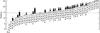 |
Fig. 1 Term energies of the target levels (54 configurations). The lowest 358 terms which produce levels having energies below the dashed line have been retained for the close-coupling expansion. |
There is now interest in various communities in estimates on the accuracy of atomic data (see, e.g. Guennou et al. 2013). There are clearly various approaches, but carrying out a large-scale calculation and comparing the resulted line intensities with those obtained from smaller targets, as we normally do, provides an indication on the uncertainty in the line intensities. Another indication on the accuracy of the atomic data comes from direct comparisons between predicted and observed line intensities. We have carried out this benchmarking process on an ion-by-ion basis for most of the iron ions (see the first paper in the series, Del Zanna et al. 2004), however some comparisons are also included here.
Our previous (jajom+ term coupling) R-matrix scattering calculation for Fe ix (Storey et al. 2002) focused on the main n = 3 levels, but also included the 3s2 3p5 4s and 3s2 3p5 4p configurations. Later, we also presented distorted wave (DW) scattering calculations which included up to n = 6 levels (O’Dwyer et al. 2012). These data have been made available via CHIANTI v.7.1 (Landi et al. 2013). A comparison between the DW and the R-matrix results showed that a significant enhancement due to resonances is present in the collision strengths to the 3s2 3p5 4s levels. The 3s2 3p5 4p levels were the highest in the previous R-matrix scattering target for Fe ix, hence we could not assess if resonances also affected these levels.
The Storey et al. (2002) and O’Dwyer et al. (2012) atomic data for Fe ix have been benchmarked against EUV and X-ray observations in Del Zanna (2009a, 2012a,b, 2013), Young (2009), O’Dwyer et al. (2012). Good overall agreement was found, suggesting that these atomic data are reasonably accurate. However, problems in the calibration of soft X-ray spectra (Del Zanna 2012a) and the EUV ones of Hinode EIS (Del Zanna 2013) have been found, hence some previous comparisons are in need of revision.
Based on the above-mentioned theoretical results, and the uncertainty in the previous benchmarks, we therefore carry out an R-matrix scattering calculation for Fe ix which improves on our previous R-matrix calculations for the n = 3 and the 3s2 3p5 4l (l = s,p), by adding the 3s2 3p5 4l (l = d, f) levels, as well as the main n = 5 configurations.
The paper is organised as follows. In Sect. 2 we outline the methods we adopted for the scattering calculations. In Sect. 3 we present our results and in Sect. 4 we reach our conclusions.
2. Methods
The atomic structure calculations were carried out using the autostructure program (Badnell 2011), which originated from the superstructure program (Eissner et al. 1974), and which constructs target wavefunctions using radial wavefunctions calculated in a scaled Thomas-Fermi-Dirac statistical model potential with a set of scaling parameters. The program also provides radiative rates and infinite energy Born limits. These limits are particularly important from two aspects. First, they allow a consistency check of the collision strengths in the scaled Burgess & Tully (1992) domain (see also Burgess et al. 1997). Second, they are used in the interpolation of the collision strengths at high energies.
The R-matrix method used in the scattering calculation is described in Hummer et al. (1993) and Berrington et al. (1995). Like the previous work on Fe ix by Storey et al. (2002), a full Breit-Pauli R-matrix (BPRM) calculation of the size we need to address the issues discussed in the introduction is impractical. Thus, we performed the calculation in the inner region in LS coupling and included mass and Darwin relativistic energy corrections. The main drawback of the (jajom+ term coupling) approach is that only the open-open part of the (physical) reactance K-matrix is transformed to take account of spin-orbit mixing in the target. The ICFT method introduced by Griffin et al. (1998) overcomes this drawback by transforming (term-coupling) the entire unphysical K-matrix utilizing multi-channel quantum defect theory for the complete closed-channel description. We note that there is an extended literature where the results of the ICFT and BPRM methods are compared. For example, the original works by Griffin et al. (1998) for Mg-like ions, and Badnell & Griffin (1999) for Ni v. More recently, Liang & Badnell (2010) carried out extensive comparisons between ICFT and DARC for Fe xvii and Kr xxvii, while Liang et al. (2009) made extensive comparisons between ICFT and DARC (and some BPRM) for Fe xvi. No significant differences between the results of the two methods have been found. The small differences that were found are within the typical spread seen in R-matrix calculations that use different configuration interaction (CI) and/or close-coupling (CC) expansions, and resonance resolution.
Dipole-allowed transitions were topped-up to infinite partial wave using an intermediate coupling version of the Coulomb-Bethe method as described by Burgess (1974) while non-dipole allowed transitions were topped-up assuming that the collision strengths form a geometric progression in J (see Badnell & Griffin 2001).
The collision strengths were extended to high energies by interpolation using the appropriate high-energy limits in the Burgess & Tully (1992) scaled domain. The high-energy limits were calculated with autostructure for both optically-allowed (see Burgess et al. 1997) and non-dipole-allowed transitions (see Chidichimo et al. 2003).
We have also carried out Breit-Pauli DW calculations using the recent development of the autostructure code, described in detail in Badnell (2011).
The temperature-dependent effective collisions strength Υ(i − j) were calculated by assuming a Maxwellian electron distribution and linear integration with the final energy of the colliding electron.
3. Results
3.1. The target
For our configuration basis set we chose the complete set of 54 configurations shown in Fig. 1 and listed in Table 1. They give rise to 1921 LS terms and 4631 fine-structure levels. The scaling parameters λnl for the potentials in which the orbital functions are calculated are also given in Table 1. The 865 fine-structure levels arising from the (energetically) lowest 358 LS terms were retained for the scattering calculation. They include all the spectroscopically important n = 4,5 levels. We note that the excitations to the last few levels may not be very accurate due to the lack of configuration interaction with absent higher configurations. We have performed both an ICFT R-matrix and a DW calculation using the same basis. They are both large-scale calculations. For example, the target of the previous R-matrix calculations (Storey et al. 2002) included only 64 LS terms from the (energetically) lowest six configurations.
Table 2 presents a selection of fine-structure target level energies Et, compared to experimental energies Eexp. A set of “best” energies Eb was obtained with a quadratic fit between the Eexp and Et values. For the observed levels, most Eb values were within 0.02 Ryd of the Eexp ones. The Eb values were used (together with the Eexp ones whenever available) within the R-matrix calculation to obtain an accurate position for the resonance thresholds. The resonances in the transitions to the n = 4 levels are close to thresholds, therefore it is important to position them as accurately as possible.
Target electron configuration basis and orbital scaling parameters λnl for the R-matrix and DW runs.
We have compared the oscillator strengths of the dipole-allowed transitions with those of the previous R-matrix calculations (Storey et al. 2002). The overview is shown in Fig. 2. Good agreement (to within ±30%) is found for transitions within the n = 3 complex (black boxes in the figure). Significant disagreements (over 100% in some cases) are found for the transitions to the n = 4 levels (red stars in the figure). The main differences, considering only the lines with the strongest oscillator strengths, occur for transitions from several levels which have the highest energies in the previous target, within the 3s2 3p4 3d2 and 3s2 3p5 4p configurations. We note that the previous target was optimized for the n = 3 levels and not the n = 4 ones, so it is not surprising to see such large discrepancies.
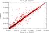 |
Fig. 2 Oscillator strengths compared to those of the Storey et al. (2002) target. Boxes: to n = 3 levels. Stars: to n = 4 levels. Dashed lines indicate ±30% differences. |
Of these transitions, only one is of relevance to astrophysical plasmas, since it is the only one with significant intensity. It involves the highest level in the previous target (Storey et al. 2002), the 13–148 3s2 3p5 3d 1P1o–3s2 3p5 4p 1S0 transition. Note that the upper level is mainly populated via a direct excitation from the ground state, then decays with this dipole-allowed transition to the lower 3s2 3p5 3d 1P1 level, which, interestingly, then decays to the ground state 3s2 3p61S0 giving rise to the resonance transition at 171 Å. The gf value for the 13–148 transition in length form is 0.19, while in velocity form is 0.10. With our previous target (Storey et al. 2002), the gf value for the same transition was 0.38 (in length; 0.14 in velocity form), i.e. almost a factor of two higher. This difference is mainly due to interaction effects among the n = 4 configurations, not taken into account in our previous target. We also note that the differences in the targets not only affect the branching ratios of the decays from the 3s2 3p5 4p 1S0 level, but also the population of this level, as discussed below.
Level energies (cm-1) for Fe ix.
Similar discrepancies in the A values for the decays from the 4p 1S0 level were also noted by Landi & Young (2009), who carried out a series of structure calculations. Their most extended target, FAC 7, is somewhat different to our present one, but produces A values in close agreement with ours, as shown in Table 3. The same table shows for comparison other A-values previously calculated. The most complete calculation of radiative rates for this ions was carried out by Aggarwal et al. (2006) with the General purpose Relativistic Atomic Structure Package (grasp). We can see that there is generally good agreement between the present values and those previously calculated by Aggarwal et al. (2006) with grasp and by Storey et al. (2002) with superstructure.
Verma et al. (2006) produced a large-scale structure calculation (including some n = 3,4,5 configurations) using Hibbert’s CIV3 Program and semi-empirical corrections to obtain a good match in level energies for the few that were known at the time. As pointed out by Aggarwal et al. (2006), the A-values calculated by Verma et al. (2006) are sometimes at odds with theirs and the Storey et al. (2002) ones, the difference likely attributable to the omission of the 3s2 3p3 3d3, which is important for configuration interaction.
3.2. The scattering calculation
The expansion of each scattered electron partial wave was done over a large basis of 35 functions within the R-matrix boundary and the partial wave expansion extended to a maximum total orbital angular momentum quantum number of L = 16. This produced accurate collision strengths up to 70 Ryd.
The outer region calculation includes exchange up to a total angular momentum quantum number J = 25/2. We have supplemented the exchange contributions with a non-exchange calculation extending from J = 27/2 to J = 73/2. The outer region exchange calculation was performed in a number of stages. The resonance region itself was calculated with an increasing number of energies, as was done for the Iron Project Fe xi calculation (Del Zanna et al. 2010). The number of energy points was increased from 800 up to 7200 (equivalent to a uniform step length of 0.00205 Ryd). A coarse energy mesh (0.57 Ryd) was chosen above all resonances, up to 70 Ryd.
We inspected all the collision strengths and their thermal averages from the ground configuration in the Burgess & Tully (1992) scaled domain. Excellent agreement between the background R-matrix and the DW collision strengths is found in all cases, as expected. Very good agreement is also found for all the strongest transitions included in the previous R-matrix calculations (Storey et al. 2002), with the exception of the 13–148 3s2 3p5 3d 1P1–3s2 3p5 4p 1S0 transition. This discrepancy was expected, considering the large differences in the gf values that we have discussed previously.
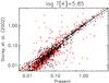 |
Fig. 3 Thermally-averaged collision strengths Υ (Storey et al. 2002 vs. the present ones) for transitions from the lowest 12 levels. Boxes: to n = 3 levels. Stars: to n = 4 levels. Dashed lines indicate ±30% differences. |
Transition probabilities for the main lines.
We calculated the thermally-averaged (effective) collision strengths, Υ, and compared them with the previous R-matrix results (Storey et al. 2002). Figure 3 shows a comparison at log Te [K] = 5.85, the temperature of peak ion abundance in ionization equilibrium, for all transitions from the lowest 12 levels. Most of these are metastable levels, hence these collisions are important in populating the higher levels. As expected, there is an overall scatter for the weaker transitions, and a marked tendency toward increased collision strengths in the present calculation, due to the extra resonances within this much larger target. If only the transitions to the n = 3 levels are considered, we see very good agreement (within ±30%) for all the stronger transitions, indicating that the extra resonances due to the n = 4,5 levels are important only for the weaker transitions. One example is shown in Fig. 4, where we compare the effective collision strengths of the two R-matrix calculations, together with the DW results. Very good agreement between the two R-matrix results is present, while the DW result is much lower, because is lacking the resonance enhancement. The following Figs. 5–8 show similar comparisons, for a sample of transitions that are of particular importance for populating levels which produce observable lines, as discussed below.
3.3. Line intensities
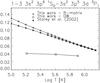 |
Fig. 4 Thermally-averaged collision strengths for the 1–3 transition (see text). |
We used the autostructure code to calculate all the transition probabilities among all the levels, for the dipole-allowed and forbidden transitions, up to third order multipoles. The experimental energies Eexp, and the best energies Eb were used when calculating the radiative rates. This is important especially for the forbidden transitions.
We then built two ion population models. The first one contained all the R-matrix excitation rates (865 fine-structure levels). The second one added excitation rates to all the extra levels that were part of the CI expansion shown in Fig. 1 and Table 1. The collision strengths to these extra levels were calculated with the DW approximation. We then solved for the level population and compared the line intensities of the two models. This was done to see if the extra configurations had any significant effect (via cascading) to the lower levels included in the CC expansion. We found no significant differences, as expected given that the extra configurations have very small collision strengths, hence have very low populations.
The relative intensities calculated with the first model, i.e. with the R-matrix excitation rates and the full set of radiative rates are shown in the third column of Table 4. Within the same table, we show in the fourth and fifth columns the corresponding intensities calculated with the Storey et al. (2002) model and with the model built by adding the n = 4,5,6 transitions as calculated in O’Dwyer et al. (2012) with the DW approximation.
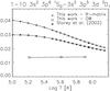 |
Fig. 5 Thermally-averaged collision strengths for the 1–10 transition (see text). |
There is overall good agreement between the three models, with most differences of the order of 10% or so. However, a few differences with the Storey et al. (2002) model are worth commenting. To establish the reasons for the differences, we have looked at which processes populate the upper levels.
The increased intensity of the decay from the 3s2 3p5 3d 3F2 level (No. 7) is mainly due to an increased A-value in the present calculation (1.9 instead of 1.3, see Table 3). We note that this level is mainly populated by cascading from higher levels. The increased intensity of the decay from the 3s2 3p5 3d 3D1 level (No. 10) is partly due to increased excitation from the ground state (see Fig. 5), partly from increased cascading. We note, in fact, that almost half of the population of level 10 is due to cascading from higher levels. We also note that the DW approximation significantly underestimates the collision strength to the 3s2 3p5 3d 3D1 level.
The slightly increased intensities of the decays from the 3s2 3p5 4s levels is mainly due to extra cascading in the larger target, which was already accounted for in our previous model (which included the DW excitation rates of O’Dwyer et al. 2012), and not due to significant changes in the collision strengths to these levels. This is because the main resonances for these levels are due to the 3s2 3p5 4p levels, which were included in the previous R-matrix calculation.
The intensity of the decay from the 3s2 3p5 4d 1P1 level (207) is increased, compared to the previous DW model of O’Dwyer et al. (2012). The population of this level is partly (30%) due to cascading from the 3s2 3p5 5p 1S0 level, and mostly (60%) by direct excitation from the ground state, which is significantly increased with the present R-matrix calculation, as shown in Fig. 6. The increase is due to the effect of the resonances.
3.4. Temperature diagnostics
The main decay form the 3s2 3p5 4p 1S0 level was identified by Young (2009) with an Hinode EIS line at 197.862 Å and our previous R-matrix calculations (Storey et al. 2002). As shown in Young (2009), the ratio of this line with the resonance line (171 Å) is in principle a good temperature diagnostic for Hinode EIS (although there is some density sensitivity). The predicted intensity of the 197.862 Å line, with the present model, is significantly (50%) lower.
The differences in the 13–148 3s2 3p5 3d 1P1–3s2 3p5 4p 1S0 transition are due to the differences in the gf value for this transition (discussed previously) and the collision strength to the 3s2 3p5 4p 1S0 from the ground state, as shown in Fig. 8.
List of the brightest Fe ix lines.
It is interesting then to reassess the comparison with Hinode EIS observations. There are, however, further complications. One is that the resonance line is barely visible, since the EIS sensitivity at 171 Å is about three orders of magnitude lower than at the peak (that is around 195 Å). Another one is that the EIS ground calibration was found to be in need of significant revisions. A new radiometric calibration was obtained by Del Zanna (2013). This calibration is very uncertain near the resonance line, however excellent agreement between predicted and observed intensities is found, as shown in Fig. 9. This figure shows the “emissivity ratio” curves  (1)for each line as a function of the electron temperature Te. Iob is the observed intensity of the line, Nj(Ne,Te) is the population of the upper level j relative to the total number density of the ion, calculated at a fixed density Ne = 109 cm-3, Aji is the spontaneous radiative transition probability, and C is a scaling constant chosen so the emissivity ratio is near unity. If agreement between experimental and theoretical intensities is present, all lines should be closely spaced. If the plasma is nearly isothermal, all curves should cross at the isothermal temperature.
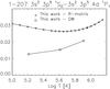 |
Fig. 6 Thermally-averaged collision strengths for the 1–207 transition (see text). Boxes indicate the DW values. |
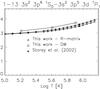 |
Fig. 7 Thermally-averaged collision strengths for the 1–13 resonance transition (see text). |
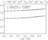 |
Fig. 8 Thermally-averaged collision strengths for the 1–148 transition (see text). |
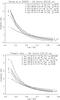 |
Fig. 9 Emissivity ratio curves relative to the “foreground-subtracted” sunspot loop leg observed by Hinode EIS (Del Zanna 2009a), using the previous (Storey et al. 2002, above) and present (below) atomic data, and the new radiometric calibration (Del Zanna 2013). The intensities Iob are in phot cm-2 s-1 arcsec-2. |
The observed intensities refer to an observation of an active region loop leg near a sunspot, where the overlying (weak) coronal emission was subtracted, leaving a very clean low-temperature spectrum (Del Zanna 2009a) with strong Fe ix lines. Some of the Fe ix lines are in fact normally blended with higher-temperature lines (see, e.g. Del Zanna 2013).
Figure 9 shows that there is better agreement between observed and predicted intensities using the new atomic data, providing a temperature of about log T[K] = 5.6, close to the temperature obtained from emission measure modelling (Del Zanna 2009b). The scaling constant for the two plots in Fig. 9 is the same, 4.5 × 10¹¹, and indeed the emissivity ratio curve for the resonance transition (No. 1, at 171 Å) is basically the same. This is because the collision strengths of the two calculations are very similar, as shown in Fig. 7. The emissivity of the 188.49 Å line (No. 2 in the figure) is also very similar in the two models. The emissivity of the 197.85 Å line (No. 3 in the figure) is instead quite different, because of the much lower A-value (see Table 3) and collision strength from the ground state (see Fig. 8), which populates the upper level. The emissivity of the 189.93 Å line (No. 4 in the figure) is slightly different, mainly because of slightly lower A-value (see Table 3). The same occurs for the 191.22 Å line (No. 5 in the figure).
3.5. Line identifications
The good agreement in the line intensity of the 13–148 transition suggests that the Young (2009) identification is correct. This level decays to the 3s2 3p5 4s 1P1, 3P1 with two UV lines that should be observable. The energy of the 4p 1S0 level is known, once the 13–148 transition is identified. The energies of the 4s 1P1, 3P1 levels are also known, because the decays to the ground state are observed, as two strong X-ray lines, at 103.564 and 105.209 Å (Behring et al. 1972). These two solar X-ray wavelengths are very close to those measured in the laboratory (Kruger et al. 1937; Fawcett et al. 1972), and should have an accuracy better than 10 mÅ.
Using the X-ray wavelengths and the Hinode EIS wavelength for the 13–148 transition measured by Young (2009) (197.862 Å), one obtains that the two main UV decays to the 4s levels should be at 804.20 and 717.13 Å. Using the Hinode EIS wavelength measured by Del Zanna (2009a) (197.854 Å) provides similar wavelengths (804.01 and 716.98 Å).
Landi & Young (2009) identified the two UV decays in SOHO SUMER spectra with lines observed at 803.42 and 717.66 Å. Using the previous atomic data, the intensity of the second line was in good agreement with the intensity of the 13–148 transition, observed by Hinode EIS. However, the 803.42 Å line was almost a factor of two too bright. With the present atomic data, the intensity of the 803.42 Å line becomes instead in excellent agreement with theory, as shown in Fig. 10, while the observed intensity of the 717.66 Å line becomes a factor of two too weak. The discrepancy in the wavelength and intensity of this weaker line is puzzling and deserves further investigations.
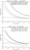 |
Fig. 10 Emissivity ratio curves for a quiet Sun Hinode/EIS and SOHO/SUMER observation described by Landi & Young (2009), using the previous (Storey et al. 2002, above) and present (below) atomic data. |
As we have discovered in the other coronal irons, the core-excited transition 3s2 3p61S0–3s 3p6 4s 1S0 is relatively strong, and the upper level decays via a strong dipole-allowed transition (3s2 3p5 3d 1P1–3s 3p6 4s 1S0, 13–256). The same type of transitions for Fe x, Fe xi, Fe xii, and Fe xiii have all been identified in Del Zanna (2012a). The differences between the target and observed wavelengths for the transitions from the n = 4 levels are about 5–6 Å, as shown in Table 4. We can therefore predict that this spectral line should fall around 146–147 Å. To identify this line, we have considered the high-resolution spectrum of Behring et al. (1972), but also that of Malinovsky & Heroux (1973), which we have scanned and recalibrated in Del Zanna (2012a).
There are several potential candidate lines in that spectral region, however most of them are due to Ni x transitions. Behring et al. (1972) lists a strong line at 146.937 Å, which could be the 13–256 Fe ix transition. However, this line is weak in the Malinovsky & Heroux (1973) spectrum. Behring et al. (1972) also lists a line at 147.274 Å, which they identify with the 2s2 2p5 2P1/2–2s 2p6 2S1/2 of Ca xii. Behring et al. (1972) identified the 141.032 Å with the 2s2 2p5 2P3/2–2s 2p6 2S1/2 of Ca xii. The theoretical branching ratio of these two Ca xii lines is 0.4, while the 147.274 Å line has about the same intensity as the 141.032 Å line. Therefore, only a fraction of the 147.274 Å line can at most be due to Ca xii, assuming that the stronger 141.032 Å line is all due to Ca xii, something that is dubious. In fact, Ca xii is formed around 3 MK, and the 141.032 Å line is expected to be very weak during moderate solar activity, as in the Malinovsky & Heroux (1973) spectrum. We therefore identify the Fe ix 3s2 3p5 3d 1P1–3s 3p6 4s 1S0 (13–256) transition with the 147.274 Å line, since it has about the predicted intensity and wavelength.
According to our ion model, several transitions from the 3s2 3p4 3d2 configuration should produce spectral lines of similar intensities as those identified by Young (2009) and therefore well visible in the Hinode EIS spectra. We have searched the Del Zanna (2009a) EIS spectrum for wavelength and intensity coincidences. Our results agree with the Young (2009) identifications, providing good agreement between predicted and observed intensities, shown in Fig. 9. The identifications of the strongest lines are summarised in Table 4 and shown in Fig. 11. The main decay from the 3D3 (5–110 transition) is one of the stronger lines from this ion. In agreement with Young & Landi (2009), we identify this transition with a line observed with Hinode EIS at 176.945 Å by Del Zanna (2009a) and at 176.959 Å by Young & Landi (2009).
According to the discussion in Del Zanna (2009a), only about half of the intensity of the 176.945 Å line is due to Fe vii. About 30% could be due to the 5–110 transition. The main decay from the 3D2 (6–111 transition) is predicted to be at 177.6 Å and indeed there is a line with the right intensity, which was identified in Young & Landi (2009).
The spectrum obtained in Del Zanna (2009a) is a pure low-temperature one, with many unidentified cool lines emitted at similar temperatures as Fe ix. We have compared predicted wavelengths and intensities for the weaker Fe ix lines with the observed ones, and suggest a few other identifications, which should be regarded as tentative. The 13–166 is a weak line, possibly blending with the Fe xi 181.10 Å line. The 8–118 is also a weak line, possibly also blended with the 176.945 Å line. The 4–85 should be well observed by EIS, with a predicted wavelength around 195 Å. There is a cool line in the spectrum at 194.784 Å, which we tentatively identify as the 4–85 transition, although it is slightly brighter than predicted, as shown in Fig. 11.
Finally, the 8–105 transition should be around 192 Å. There are two options, an unidentified cool line at 192.094 Å, or a line blending with Fe xi (see the identifications of this ion discussed in Del Zanna 2010) at 192.630 Å. We choose the second option, because it has a difference with the predicted wavelength closer to the differences of the other lines of the same transition array.
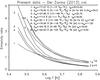 |
Fig. 11 Emissivity ratio curves relative to a few newly identified lines in the Hinode EIS spectra (as in Fig. 9). |
3.6. Electron density diagnostics
There are several excellent line ratios in Fe ix that can be used to measure electron densities. The best is the ratio of the strong and nearby lines at 241.7 and 244.9 Å. This ratio, as well as the ratios involving the 217. Å line, were discussed in Storey et al. (2002) and are not further considered here.
We would instead like to point out here the usefulness of the visible forbidden lines to measure electron densities. Fe ix produces several strong forbidden lines, which, after several attempts, were finally identified by Edlen & Smitt (1978). Earlier literature estimated the intensities of these lines, and found several large inconsistencies (up to factors of two) with the observed values (see, e.g. Haug 1979). It is therefore interesting to revisit this issue with the present data. We consider one of the very few observations of these lines, a ground-based one obtained in 1965 May 30 during a total solar eclipse by Jefferies et al. (1971). We selected the calibrated intensities of the lines observed close to the solar limb above a so-called coronal condensation, and plot in Fig. 12 the emissivity ratio curves for all the measured lines.
We can see that the curves for the 3800.8 and 4585.3 Å lines (Nos. 1 and 4 in the plot) are very close, hence there is very good agreement between predicted and observed intensities for these lines, which form a branching ratio. The curve for the 4359.4 Å line, which was incorrectly identified as due to Ni xiii by Jefferies et al. (1971), intersects the previous two lines around 108 cm-3, while the 3642.7 Å would provide a higher electron density, around 108.8 cm-3. The 3642.7 and 4359.4 Å lines also form a branching ratio, which we expect to be quite accurate. Therefore, either the observed intensity of the 3642.7 Å line was overestimated, or the intensity of the 4359.4 Å line underestimated by about 40%. In any case, all the intensities are, within ±20%, in agreement.
We thought at first that a density of 108 cm-3 was perhaps too low, being closer to a quiet Sun rather than a coronal condensation (which is normally associated with active regions), so we revisited other density diagnostics from the same observation. The only other reliable density diagnostics at similar temperatures is given by the forbidden lines of Fe x. Our earlier R-matrix calculations showed significant discrepancies with observations (Del Zanna et al. 2004), as Fig. 13 (top plot) shows. However, our recent large-scale R-matrix calculations for Fe x (Del Zanna et al. 2012b) show quite a different picture. As Fig. 13 (bottom plot) shows, good agreement (to within ±20%) is found, indicating electron densities of about 108 cm-3 (or less), i.e. similar to what obtained from the Fe ix 4359.4 Å line.
A quick comparison of the two plots in Fig. 13 (obtained with the same scaling constant) shows that the red forbidden line (No. 1) has a very similar emissivity, using the old and the new atomic data. Indeed, as shown in Del Zanna et al. (2012b), the collision strength for this important transition is very close that what was previously calculated. On the other hand, the emissivities of all the other forbidden lines are increased by a factor of two or more with the last calculation. This ultimately is due to the combined effect of increased collision strengths and cascading, an important issue that was not highlighted in the Fe x paper, but was discussed in detail for Fe xi (Del Zanna et al. 2010) and Fe xii (Del Zanna et al. 2012a).
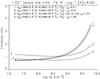 |
Fig. 12 Emissivity ratio curves of the coronal forbidden lines observed by Jefferies et al. (1971), for Fe ix using the present atomic data. The dashed lines indicate ±20%. |
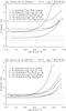 |
Fig. 13 Emissivity ratio curves of the coronal forbidden lines observed by Jefferies et al. (1971), for Fe x using the earlier data (Del Zanna et al. 2004), above, and the most recent ones (Del Zanna et al. 2012b) below. The dashed lines indicate ±20%. |
4. Summary and conclusions
In many respects, the present large-scale calculations have produced results similar to those of the other coronal iron ions that we have carried out. For most of the strongest lines, agreement within a few percent in the line intensities calculated at peak ion abundance in equilibrium is found. This confirms the accuracy of the calculations for strong transitions.
The collision strengths to the n = 3 levels are not significantly different compared to our previous calculation. This means that the present large-scale target is not necessary, if one is only interested in n = 3 transitions.
Notable enhancements in the weaker transitions are however present, due to the extra resonances in the larger target. Compared to the previous ion model, which included R-matrix (Storey et al. 2002) and DW (O’Dwyer et al. 2012) calculations, significant increases are only found for transitions to the 4d levels, because of the resonance enhancement, compared to the DW calculations. Resonance excitation to the 4s levels is also important, but was already included in our previous R-matrix calculations.
As for the other coronal iron ions, we have found that transitions from levels populated via a core-excited transition are quite strong, and provided a new identification for Fe ix as a soft X-ray line at 147.274 Å.
The predicted intensities of some among the strongest Fe ix EUV lines, observed by Hinode EIS, are now in much
better agreement with observations, providing a reliable way to measure electron temperatures for the solar corona. We have provided a few further identifications (some will need to be confirmed with laboratory spectroscopy) of lines observed by Hinode EIS. Some identifications, in particular those of the lines observed by SUMER, need further investigation. Fe ix lines can also be reliably used to measure electron densities. Very good diagnostics are provided by EUV and visible lines.
Acknowledgments
The present work was funded by STFC (UK) through the University of Cambridge DAMTP astrophysics grant, and the University of Strathclyde UK APAP network grant ST/J000892/1. We thank the anonymous referee for useful suggestions, and E. Landi for providing unpublished A-values.
References
- Aggarwal, K. M., Keenan, F. P., Kato, T., & Murakami, I. 2006, A&A, 460, 331 [NASA ADS] [CrossRef] [EDP Sciences] [Google Scholar]
- Badnell, N. R. 2011, Comp. Phys. Comm., 182, 1528 [Google Scholar]
- Badnell, N. R., & Griffin, D. C. 1999, J. Phys. B At. Mol. Phys., 32, 2267 [NASA ADS] [CrossRef] [Google Scholar]
- Badnell, N. R., & Griffin, D. C. 2001, J. Phys. B At. Mol. Phys., 34, 681 [NASA ADS] [CrossRef] [Google Scholar]
- Behring, W. E., Cohen, L., & Feldman, U. 1972, ApJ, 175, 493 [NASA ADS] [CrossRef] [Google Scholar]
- Berrington, K. A., Eissner, W. B., & Norrington, P. H. 1995, Comp. Phys. Comm., 92, 290 [Google Scholar]
- Burgess, A. 1974, J. Phys. B At. Mol. Phys., 7, L364 [NASA ADS] [CrossRef] [Google Scholar]
- Burgess, A., & Tully, J. A. 1992, A&A, 254, 436 [NASA ADS] [Google Scholar]
- Burgess, A., Chidichimo, M. C., & Tully, J. A. 1997, J. Phys. B At. Mol. Phys., 30, 33 [NASA ADS] [CrossRef] [Google Scholar]
- Chidichimo, M. C., Badnell, N. R., & Tully, J. A. 2003, A&A, 401, 1177 [NASA ADS] [CrossRef] [EDP Sciences] [Google Scholar]
- Culhane, J. L., Harra, L. K., James, A. M., et al. 2007, Sol. Phys., 60 [Google Scholar]
- Del Zanna, G. 2009a, A&A, 508, 501 [NASA ADS] [CrossRef] [EDP Sciences] [Google Scholar]
- Del Zanna, G. 2009b, A&A, 508, 513 [NASA ADS] [CrossRef] [EDP Sciences] [Google Scholar]
- Del Zanna, G. 2010, A&A, 514, A41 [NASA ADS] [CrossRef] [EDP Sciences] [Google Scholar]
- Del Zanna, G. 2012a, A&A, 546, A97 [NASA ADS] [CrossRef] [EDP Sciences] [Google Scholar]
- Del Zanna, G. 2012b, A&A, 537, A38 [NASA ADS] [CrossRef] [EDP Sciences] [Google Scholar]
- Del Zanna, G. 2013, A&A, 555, A47 [NASA ADS] [CrossRef] [EDP Sciences] [Google Scholar]
- Del Zanna, G., & Storey, P. J. 2013, A&A, 549, A42 [NASA ADS] [CrossRef] [EDP Sciences] [Google Scholar]
- Del Zanna, G., Berrington, K. A., & Mason, H. E. 2004, A&A, 422, 731 [NASA ADS] [CrossRef] [EDP Sciences] [Google Scholar]
- Del Zanna, G., Storey, P. J., & Mason, H. E. 2010, A&A, 514, A40 [NASA ADS] [CrossRef] [EDP Sciences] [Google Scholar]
- Del Zanna, G., Storey, P. J., Badnell, N. R., & Mason, H. E. 2012a, A&A, 543, A139 [NASA ADS] [CrossRef] [EDP Sciences] [Google Scholar]
- Del Zanna, G., Storey, P. J., Badnell, N. R., & Mason, H. E. 2012b, A&A, 541, A90 [NASA ADS] [CrossRef] [EDP Sciences] [Google Scholar]
- Edlen, B., & Smitt, R. 1978, Sol. Phys., 57, 329 [NASA ADS] [CrossRef] [Google Scholar]
- Eissner, W., Jones, M., & Nussbaumer, H. 1974, Comp. Phys. Comm., 8, 270 [Google Scholar]
- Fawcett, B. C., Peacock, N. J., & Cowan, R. D. 1968, J. Phys. B At. Mol. Phys., 1, 295 [NASA ADS] [CrossRef] [Google Scholar]
- Fawcett, B. C., Kononov, E. Y., Hayes, R. W., & Cowan, R. D. 1972, J. Phys. B At. Mol. Phys., 5, 1255 [Google Scholar]
- Griffin, D. C., Badnell, N. R., & Pindzola, M. S. 1998, J. Phys. B At. Mol. Phys., 31, 3713 [NASA ADS] [CrossRef] [Google Scholar]
- Guennou, C., Auchère, F., Klimchuk, J. A., Bocchialini, K., & Parenti, S. 2013, ApJ, 774, 31 [NASA ADS] [CrossRef] [Google Scholar]
- Haug, E. 1979, Sol. Phys., 61, 311 [NASA ADS] [CrossRef] [Google Scholar]
- Hummer, D. G., Berrington, K. A., Eissner, W., et al. 1993, A&A, 279, 298 [NASA ADS] [Google Scholar]
- Jefferies, J. T., Orrall, F. Q., & Zirker, J. B. 1971, Sol. Phys., 16, 103 [NASA ADS] [CrossRef] [Google Scholar]
- Kruger, P. G., Weissberg, S. G., & Phillips, L. W. 1937, Phys. Rev., 51, 1090 [NASA ADS] [CrossRef] [Google Scholar]
- Landi, E., & Young, P. R. 2009, ApJ, 707, 1191 [NASA ADS] [CrossRef] [Google Scholar]
- Landi, E., Young, P. R., Dere, K. P., Del Zanna, G., & Mason, H. E. 2013, ApJ, 763, 86 [NASA ADS] [CrossRef] [Google Scholar]
- Liang, G. Y., & Badnell, N. R. 2010, A&A, 518, A64 [NASA ADS] [CrossRef] [EDP Sciences] [Google Scholar]
- Liang, G. Y., Whiteford, A. D., & Badnell, N. R. 2009, A&A, 500, 1263 [NASA ADS] [CrossRef] [EDP Sciences] [Google Scholar]
- Malinovsky, L., & Heroux, M. 1973, ApJ, 181, 1009 [NASA ADS] [CrossRef] [Google Scholar]
- O’Dwyer, B., Del Zanna, G., Badnell, N. R., Mason, H. E., & Storey, P. J. 2012, A&A, 537, A22 [NASA ADS] [CrossRef] [EDP Sciences] [Google Scholar]
- Storey, P. J., Zeippen, C. J., & Le Dourneuf, M. 2002, A&A, 394, 753 [NASA ADS] [CrossRef] [EDP Sciences] [Google Scholar]
- Verma, N., Jha, A. K. S., & Mohan, M. 2006, ApJS, 164, 297 [NASA ADS] [CrossRef] [Google Scholar]
- Young, P. R. 2009, ApJ, 691, L77 [NASA ADS] [CrossRef] [Google Scholar]
- Young, P. R., & Landi, E. 2009, ApJ, 707, 173 [NASA ADS] [CrossRef] [Google Scholar]
All Tables
Target electron configuration basis and orbital scaling parameters λnl for the R-matrix and DW runs.
All Figures
|
Fig. 1 Term energies of the target levels (54 configurations). The lowest 358 terms which produce levels having energies below the dashed line have been retained for the close-coupling expansion. |
| In the text | |
|
Fig. 2 Oscillator strengths compared to those of the Storey et al. (2002) target. Boxes: to n = 3 levels. Stars: to n = 4 levels. Dashed lines indicate ±30% differences. |
| In the text | |
|
Fig. 3 Thermally-averaged collision strengths Υ (Storey et al. 2002 vs. the present ones) for transitions from the lowest 12 levels. Boxes: to n = 3 levels. Stars: to n = 4 levels. Dashed lines indicate ±30% differences. |
| In the text | |
|
Fig. 4 Thermally-averaged collision strengths for the 1–3 transition (see text). |
| In the text | |
|
Fig. 5 Thermally-averaged collision strengths for the 1–10 transition (see text). |
| In the text | |
|
Fig. 6 Thermally-averaged collision strengths for the 1–207 transition (see text). Boxes indicate the DW values. |
| In the text | |
|
Fig. 7 Thermally-averaged collision strengths for the 1–13 resonance transition (see text). |
| In the text | |
|
Fig. 8 Thermally-averaged collision strengths for the 1–148 transition (see text). |
| In the text | |
|
Fig. 9 Emissivity ratio curves relative to the “foreground-subtracted” sunspot loop leg observed by Hinode EIS (Del Zanna 2009a), using the previous (Storey et al. 2002, above) and present (below) atomic data, and the new radiometric calibration (Del Zanna 2013). The intensities Iob are in phot cm-2 s-1 arcsec-2. |
| In the text | |
|
Fig. 10 Emissivity ratio curves for a quiet Sun Hinode/EIS and SOHO/SUMER observation described by Landi & Young (2009), using the previous (Storey et al. 2002, above) and present (below) atomic data. |
| In the text | |
|
Fig. 11 Emissivity ratio curves relative to a few newly identified lines in the Hinode EIS spectra (as in Fig. 9). |
| In the text | |
|
Fig. 12 Emissivity ratio curves of the coronal forbidden lines observed by Jefferies et al. (1971), for Fe ix using the present atomic data. The dashed lines indicate ±20%. |
| In the text | |
|
Fig. 13 Emissivity ratio curves of the coronal forbidden lines observed by Jefferies et al. (1971), for Fe x using the earlier data (Del Zanna et al. 2004), above, and the most recent ones (Del Zanna et al. 2012b) below. The dashed lines indicate ±20%. |
| In the text | |
Current usage metrics show cumulative count of Article Views (full-text article views including HTML views, PDF and ePub downloads, according to the available data) and Abstracts Views on Vision4Press platform.
Data correspond to usage on the plateform after 2015. The current usage metrics is available 48-96 hours after online publication and is updated daily on week days.
Initial download of the metrics may take a while.