| Issue |
A&A
Volume 565, May 2014
|
|
|---|---|---|
| Article Number | A119 | |
| Number of page(s) | 4 | |
| Section | Stellar structure and evolution | |
| DOI | https://doi.org/10.1051/0004-6361/201323183 | |
| Published online | 21 May 2014 | |
Research Note
Effects of moderate abundance changes on the atmospheric structure and colours of Mira variables
1 Zentrum für Astronomie der Universität Heidelberg (ZAH), Institut für Theoretische Astrophysik, Albert-Ueberle-Str. 2, 69120 Heidelberg, Germany
e-mail: This email address is being protected from spambots. You need JavaScript enabled to view it.
2 Sydney Institute for Astronomy (SIfA), School of Physics, University of Sydney, Sydney NSW 2006, Australia
3 Department of Physics and Astronomy, Macquarie University, North Ryde, Sydney NSW 2109, Australia
4 Australian Astronomical Observatory, Epping, Sydney NSW 1710, Australia
e-mail: This email address is being protected from spambots. You need JavaScript enabled to view it.
5 Research School of Astronomy and Astrophysics, Australian National University, Canberra ACT 2600, Australia
e-mail: This email address is being protected from spambots. You need JavaScript enabled to view it.
Received: 4 December 2013
Accepted: 24 April 2014
Abstract
Aims. We study the effects of moderate deviations from solar abundances upon the atmospheric structure and colours of typical Mira variables.
Methods. We present two model series of dynamical opacity-sampling models of Mira variables which have (1) 1/3 solar metallicity; and (2) “mild” S-type C/O abundance ratio ([C/O] = 0.9) with typical Zr enhancement (solar +1.0). These series are compared to a previously studied solar-abundance series which has similar fundamental parameters (mass, luminosity, period, radius) that are close to those of o Cet.
Results. Both series show noticeable effects of abundance upon stratifications and infrared colours but cycle-to-cycle differences mask these effects at most pulsation phases, with the exception of a narrow-water-filter colour near minimum phase.
Key words: stars: AGB and post-AGB / stars: atmospheres / stars: abundances
© ESO, 2014
1. Introduction
The density stratification of upper atmospheric layers of Mira variables is determined by outwards travelling shock fronts. These shock fronts are seen in typical emission lines of hydrogen and other atoms (Fox et al. 1984; Richter & Wood 2004) and lead to a geometrically very extended stellar atmosphere resulting in strong dependence of the Mira diameter observed in different absorption features (e.g. Ireland et al. 2004; Woodruff et al. 2008, 2009; Zhao-Geisler et al. 2012).
Models based on sophisticated treatment of radiative transfer have become available in recent years (Höfner et al. 2003; Ireland et al. 2008 (CODEX1), 2011 (CODEX2)). The CODEX model series, which are based upon a self-excited pulsation model for each series, show that differences in position and strength of outwards travelling – or sometimes receding – shock fronts in different cycles may lead to noticeable cycle-to-cycle differences of density and temperature in upper layers and to differences of spectral features formed in these layers. Comparison of these models with observations of Miras were published by Woodruff et al. (2009), Wittkowski et al. (2011), Hillen et al. (2012).
CODEX models have so far been computed for 4 different sets of parameters given by 4 non-pulsating “parent stars” (series R52, C50, C81, o54; see Table 1). Solar element abundances (Z = 0.02; Grevesse et al. 1996) were adopted for all series. Details of constructing pulsation models and of computing atmospheric temperatures and spectra, based upon an opacity-sampling treatment of absorption coefficients, are given in Ireland et al. (2008, 2011). In this paper, we construct two CODEX model series with (i) “mildly” sub-solar metallicity and; (ii) “mild” S-type C/O abundance ratio. In order to look for abundance-dependent differences, we compare stratifications and colours of these models with those of models of the o54 series which has, except for abundances, almost identical parameters.
We note that intermediate-period Mira variables are most typically associated with the thick disk (Groenewegen & Blommaert 2006) which does not have solar abundances and, in particular, has [Ti/Fe] enhancement of +0.2 and [O/Fe] and [C/Fe] enhancements of +0.3 to +0.4 (e.g. Reddy et al. 2006). Assuming a standard [α/Fe] = 0.0, our chosen metallicity Z = 0.02/3 corresponds to [Ti/H] = –0.5, [O/H] = –0.5 and [C/H] = –0.5. Given that Ti, O and C are the heavy elements that most significantly influence the spectra of O-rich Mira variables, the metallicity Z = 0.02/3 can thus approximately represent a thin-disk star of [Fe/H] = −0.5 as well as a thick-disk star with typical α-enhancement of +0.3 and with [Fe/H] = −0.8. This range is typical of stars kinematically associated with the thick disk (e.g. Adibekyan et al. 2011; Cheng et al. 2012). Of course, significant abundance variations are still expected throughout the intermediate-period Mira variable population. This study attempts to look for simple observational effects of these variations.
2. Model parameters and descriptions
Inspection of the models presented in Ireland et al. (2011) shows that the luminosity L, the τRoss = 1 Rosseland radius R, and the positions and heights of atmospheric shock fronts can all differ noticeably in different cycles. This leads to different effective temperatures Teff ∝ (L/R2)1/4 and to different atmospheric temperature-density stratifications for models at the same phase in different cycles. We shall investigate in this study whether typical effects of moderately lower metallicity and moderately higher S-type C/O ratio are strong enough to overcome cycle-to-cycle differences which show up in standard spectral colours. The o54 model series, assumed to have parameters close to o Cet (cf. Ireland et al. 2008, for details), is adopted as the solar-abundance reference series in the present study. The two new model series are:
-
(i)
The x54 series (see Table 1), withZ = 0.02/3, is the low-metallicity counterpart of the o54 series. The basic parent-star parameters, the period and the turbulent-velocity parameter of the x54 series are almost identical to the o54 values. And the mixing-length parameter (2.36) is somewhat lower than the o54 value (3.5), which compensates for the lower metallicity in order to match the observed period for given model luminosity and mass. The lower mixing-length parameter represents less efficient convection, increasing the stellar radius, while the lower metallicity lowers opacity, making it easier for radiation to escape, and decreases the stellar radius. A detailed discussion of these effects is given in Ireland et al. (2008, 2011).
-
(ii)
The s54 series (see Table 1) represents the “mild” S-type counterpart of the o54 series with a C enhancement of +0.274, resulting in [C/O] = 0.9, and with a Zr enhancement of +1.0 with respect to the solar values given in Grevesse et al. (1996). Since the grey pulsation model is hardly affected by such “mild” CNO changes (Teff changes by only ~10 K for fixed M, L and P), the pressure stratification of the original o54 grey pulsation model was adopted for calculating the s54 non-grey atmospheric temperature stratification and spectrum with the S-type opacities.
The behaviour of the x54 pulsation model series is shown in Fig. 1. Two time intervals, covering 3 cycles, were selected for computing atmospheric stratifications and they are marked as blue-shaded regions. Basic parameters of the models of these 3 cycles, as well as shock-front positions, are given in Table 2.
The behaviour of the solar-abundance o54 pulsation model, used for computing the S-type s54 series in the present paper, is shown in Fig. 1 and in Tables 2 to 4 of Ireland et al. (2011). Three sub-intervals comprising 3 cycles with different phase-dependent characteristics (L, R, Teff, shock front position/height) were chosen for computing S-type atmospheric stratifications. It turns out that Rosseland radii R – and resulting effective temperatures Teff – at a given phase are almost identical in s54 and o54 models except around phase 0.6 where s54 radii are moderately smaller (by about 0.2 parent-star radii) and effective temperatures are moderately higher (by about 200 K) than o54 values.
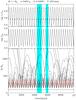 |
Fig. 1 Luminosity L, effective temperature Teff and radius R of a representative selection of mass zones plotted against time t for the low-metallicity model series x54. The red line in the R panel shows the position of the grey-approximation optical depth τg = 2/3. Teff in the grey pulsation model is defined as the temperature at τg = 2/3 and is close to the effective temperature ∝ (L/R2)1/4 of the non-grey atmospheric stratification. The blue-shaded regions show the time intervals in which models were selected for computing detailed atmospheres (shown as red circles in the L panel). |
Parameters of the x54 models including positions of shock fronts.
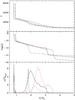 |
Fig. 2 Temperature T (upper), density ρ (middle) and density ρmol of water molecules H2O (lower panel) as a function of radius R/Rp for 4 phase 0.80 models: metal-poor x54 series (black full line), solar-abundance o54 series (green dashed, red short-dashed), S-type s54 series (blue dotted). |
3. Abundance effects on temperature stratifications
Comparison of the effective temperatures of the metal-poor x54 models (Table 2) with those of o54 models (Tables 2 to 4 of Ireland et al. 2011) shows that, despite occasionally significant luminosity differences at some phases, effective temperatures at a given phase are very similar in both series. This means that Teff ∝ (L/R2)1/4 as a function of phase hardly changes with moderately decreasing metallicity. Only around phase 0.4 can a very modest trend towards somewhat higher x54 effective temperatures (about 100 to 200 K) be seen.
When comparing the S-type s54 models with the o54 models, we are dealing with strictly differential effects caused by the CNO abundance differences between s54 and o54 (since the s54 models are based upon the pressure stratifications of the corresponding models in the o54 series). At most phases, no systematic difference between s54 and o54 effective temperatures can be found, except around phase 0.6 where the s54 model in a given cycle tends to be hotter by about 200 K than its o54 counterpart, but cycle-to-cycle differences still lead to marginal Teff overlaps.
Since the temperature stratification of the middle to upper atmosphere of a Mira variable tends to depend, at a given phase, more on the positions of shock fronts (and their associated density stratification) than on the exact value of Teff, we have to accept that modest cycle-dependent changes of Teff ∝ (L/R2)1/4 cannot be safely derived from observations of spectral features formed in these layers.
Figure 2 shows stratifications of temperature, density and H2O molecular density at phase 0.8 for a typical model of the x54 series, for 2 typical models (of different cycles) of the o54 series, and for the s54 counterpart of one of these o54 models. Cycle-to-cycle differences of the atmospheric stratification as shown, e.g., in Fig. 2 for two o54 models lead to significant spectrum differences (cf. Ireland et al. 2011). These interfere with differences caused by changing element abundances and may, of course, affect the assignment of colours to abundances.
4. Abundance effects on colours
From the findings discussed in Sect. 3, we would not expect to see really significant abundance-related spectrum differences between our model series. This is confirmed by systematic inspection of standard infrared colour indices J − H, J − K and H − K in all models which were investigated in this study. We added a set of 3 colour indices that combines JHK with a “water colour” W, defined by the flux in a narrow water-dominated bandpass (rectangular profile) centred at 1.45 μm with full width 0.087 μm. These colour indices, too, do not show clear abundance effects. (Inspection of fluxes in the I bandpass and in the optical R and V bandpasses shows still more pronounced cycle-to-cycle differences so these colours could be a priori excluded as useful abundance indicators.)
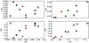 |
Fig. 3 2-colour-diagrams of (H-K) (upper panel) and (J-W) (lower panel) vs. (J-H). Left panel: phase 0.8 models of the o54 series (filled green circles), the x54 series (filled red triangles) and the s54 series (black circles). Right panel: the same as the left panel but for phase 0.6 models. |
The left panel of Fig. 3 shows 2-colour-diagrams (H − K) vs. (J − H) and (J − W) vs. (J − H) for all phase 0.8 models of this study. The stratifications of four of these models are shown in Fig. 2. No clear separation of x54, o54 and s54 models can be seen in this figure: cycle-to-cycle stratification differences clearly dominate abundance effects. This behaviour holds for the models at all pulsation phases except for models near phase 0.6 where some systematic differences between models of different abundances can be seen in the 2-colour diagrams (right panel of Fig. 3). Inspection of Table 1 of this paper and of Tables 2 to 4 of Ireland et al. (2011) shows that the effective temperature at near-minimum phase 0.6 is substantially lower than at neighbouring phases so that the influence of relevant molecules (especially water) upon the stratification and the spectrum is noticeably higher than at slightly later and, in particular, slightly earlier phases (where phase details somewhat depend on specific stellar parameters: cf. Tables 2 to 8 of Ireland et al. 2011). A careful observational campaign covering phases near minimum in small phase steps of, e.g., 0.05 would be needed to clearly see this effect in real stars. It is also important that, when making conclusions about abundances from a model series, this series must have parameters that match broadband colours, pulsation period and amplitude.
We also inspected the phase and cycle dependence of other water features, e.g. in the K band range, and found similar, but sometimes less pronounced and less obvious, abundance effects as in the W band. Colours using this band appear to be preferable abundance indicators.
One also has to be aware that the CODEX models have so far been compared to only a few stars, with more or less accurately known stellar parameters, at selected phases/cycles in selected wavelength ranges. Woodruff et al. (2009) compare fluxes and diameters of 3 stars (W Hya, R Leo, o Cet; 2 phases) in the 1.0 to 4.0 μm range with o54 models and find satisfactory agreement with some differences at longer wavelengths. Wittkowski et al. (2011) compare fluxes and visibilities/diameters of 4 stars (R Cnc, X Hya, W Vel, RW Vel; 1 phase) in the 1.9 to 2.5 μm range with models (C50, o54, C81, o54, respectively) and find satisfactory agreement with only moderate differences, although the measured closure phases indicate noticeable deviations from spherical symmetry not considered in the spherical CODEX models. Hillen et al. (2012) compare fluxes and visibilities of TU And in the 2.0 to 2.4 μm range for a large number of phases of 8 successive cycles with predictions of R52 (and o54) models. The TU And observations are well reproduced by the models at near-minimum phases but suggest that this star’s atmosphere is more extended than the model atmosphere at near-maximum phases. If this indicates a general model problem, rather than imperfect stellar vs. model parameter assignment, the present study might underestimate abundance effects on colours near maximum phases.
It might appear astonishing at first glance that “mild” changes of abundances, in particular lowering metallicity, results in only fairly small effects upon colours which can hardly be disentangled from cycle-to-cycle differences of the atmospheric structure. One has to be aware, however, that hydrogen is not a major absorber in the upper layers of such very cool atmospheres. Decreasing the metal-to-hydrogen ratio affects essentially 2 absorbers, H− and H2O, where electrons in H− come from metals, and the resulting changes of the temperature stratification (cf. Fig. 2) and of the emitted spectrum are very modest.
5. Concluding remarks
We computed two model series which allow the study of the effects of “mild” deviations from solar element abundances upon the atmospheric stratification and standard spectral colours of typical (o Cet-like) Mira variables. The x54 model series is the  metallicity counterpart of the solar-metallicity o54 series discussed by Ireland et al. (2008, 2011), while the s54 model series is the S-type counterpart of the o54 series. Both model series show noticeable stratification and spectral-colour differences from the o54 models.
It turns out, however, that such abundance effects are readily masked by significant cycle-to-cycle differences at most phases. Also, in real stars, one needs to consider in addition the effects caused by modest differences of stellar parameters, so one has to conclude that “mild” deviations from solar element abundances will barely be detectable in the structure of the stellar atmosphere and the broadband emitted spectral flux. This confirms the findings of Scholz & Wood (2004) who infer, based on a series of less elaborated models, that there is no easy way to determine the metallicity of an M-type Mira field star for moderate deviations (factor of the order of 2) from solar metallicity. We suggest that future observational campaigns should both focus on phase-dependent measurements in the W water filter and on high-spectral-resolution bandpasses that include a continuum (e.g. J and H bands) and where the classical method of line analysis can be attempted.
References
- Adibekyan, V. Zh., Santos, N. C., Sousa, S. G., & Israelian, G. 2011, A&A, 535, L11 [NASA ADS] [CrossRef] [EDP Sciences] [Google Scholar]
- Cheng, J. Y., Rockosi, C. M., Morrison, H. L., et al. 2012, ApJ, 746, 149 [NASA ADS] [CrossRef] [Google Scholar]
- Fox, M. W., Wood, P. R., & Dopita, M. A. 1984, ApJ, 286, 337 [NASA ADS] [CrossRef] [Google Scholar]
- Grevesse, N., Noels, A., & Sauval, A. J. 1996, in Cosmic Abundances, eds. S. S. Holt, & G. Sonneborn, ASP Conf. Ser., 99, 117 [Google Scholar]
- Groenewegen, M. A. T., & Blommaert, J. A. D. L. 2006, Mem. Soc. Astron. Ital., 77, 81 [NASA ADS] [Google Scholar]
- Hillen, M., Verhoelst, T., Degroote, P., Acke, B., & Van Winckel, H. 2012, A&A, 538, L6 [NASA ADS] [CrossRef] [EDP Sciences] [Google Scholar]
- Höfner, S., Gautschy-Loidl, R., Aringer, B., & Jørgensen, U. G. 2003, A&A, 399, 589 [NASA ADS] [CrossRef] [EDP Sciences] [Google Scholar]
- Ireland, M. J., Tuthill, P. G., Bedding, T. R., Robertson, J. G., & Jacob, A. P. 2004, MNRAS, 350, 365 [NASA ADS] [CrossRef] [Google Scholar]
- Ireland, M. J., Scholz, M., & Wood, P. R. 2008, MNRAS, 391, 1994 [NASA ADS] [CrossRef] [Google Scholar]
- Ireland, M. J., Scholz, M., & Wood, P. R. 2011, MNRAS, 418, 114 [NASA ADS] [CrossRef] [Google Scholar]
- Reddy, B. E., Lambert, D. L., & Allen de Prieto, C. 2006, MNRAS, 367, 1329 [NASA ADS] [CrossRef] [Google Scholar]
- Richter, He., & Wood, P. R. 2001, A&A, 369, 1027 [NASA ADS] [CrossRef] [EDP Sciences] [Google Scholar]
- Scholz, M., & Wood, P. R. 2004, in Variable Stars in the Local Group, eds. D. W. Kurtz, & K. Pollard, IAU Coll. 193, ASP Conf. Ser., 310, 313 [Google Scholar]
- Wittkowski, M., Boboltz, D. A., Ireland, M. J., et al. 2011, A&A, 532, L7 [NASA ADS] [CrossRef] [EDP Sciences] [Google Scholar]
- Woodruff, H. C., Tuthill, P. G., Monnier, J. D., et al. 2008, ApJ, 673, 418 [NASA ADS] [CrossRef] [Google Scholar]
- Woodruff, H. C., Ireland, M. J., Tuthill, P. G., et al. 2009, ApJ, 691, 1328 [NASA ADS] [CrossRef] [Google Scholar]
- Zhao-Geisler, R., Quirrenbach, A., Köhler, R., & Lopez, B. 2012, A&A, 545, A56 [NASA ADS] [CrossRef] [EDP Sciences] [Google Scholar]
All Tables
All Figures
|
Fig. 1 Luminosity L, effective temperature Teff and radius R of a representative selection of mass zones plotted against time t for the low-metallicity model series x54. The red line in the R panel shows the position of the grey-approximation optical depth τg = 2/3. Teff in the grey pulsation model is defined as the temperature at τg = 2/3 and is close to the effective temperature ∝ (L/R2)1/4 of the non-grey atmospheric stratification. The blue-shaded regions show the time intervals in which models were selected for computing detailed atmospheres (shown as red circles in the L panel). |
| In the text | |
|
Fig. 2 Temperature T (upper), density ρ (middle) and density ρmol of water molecules H2O (lower panel) as a function of radius R/Rp for 4 phase 0.80 models: metal-poor x54 series (black full line), solar-abundance o54 series (green dashed, red short-dashed), S-type s54 series (blue dotted). |
| In the text | |
|
Fig. 3 2-colour-diagrams of (H-K) (upper panel) and (J-W) (lower panel) vs. (J-H). Left panel: phase 0.8 models of the o54 series (filled green circles), the x54 series (filled red triangles) and the s54 series (black circles). Right panel: the same as the left panel but for phase 0.6 models. |
| In the text | |
Current usage metrics show cumulative count of Article Views (full-text article views including HTML views, PDF and ePub downloads, according to the available data) and Abstracts Views on Vision4Press platform.
Data correspond to usage on the plateform after 2015. The current usage metrics is available 48-96 hours after online publication and is updated daily on week days.
Initial download of the metrics may take a while.