| Issue |
A&A
Volume 564, April 2014
|
|
|---|---|---|
| Article Number | A137 | |
| Number of page(s) | 5 | |
| Section | Cosmology (including clusters of galaxies) | |
| DOI | https://doi.org/10.1051/0004-6361/201322606 | |
| Published online | 18 April 2014 | |
Cosmological model of the interaction between dark matter and dark energy
1 School of Astronomy and Space Science, Nanjing University, Nanjing 210093, PR China
2 Key Laboratory of Modern Astronomy and Astrophysics (Nanjing University), Ministry of Education, Nanjing 210093, PR China
e-mail: This email address is being protected from spambots. You need JavaScript enabled to view it.
Received: 4 September 2013
Accepted: 16 March 2014
Abstract
We tested a cosmological model for the interaction between dark matter and dark energy with a dynamic equation of state wDE(z) = w0 + w1z/ (1 + z), using type Ia supernovae (SNe Ia), Hubble parameter data, baryonic acoustic oscillation (BAO) measurements, and cosmic microwave background (CMB) observations. This interacting cosmological model has not been studied before. The best-fit parameters with 1σ uncertainties are δ = − 0.022 ± 0.006, Ω0DM = 0.213 ± 0.008, w0 = − 1.210 ± 0.033 and w1 = 0.872 ± 0.072 with χ2min/d.o.f. = 0.990. At the 1σ confidence level, we find δ < 0, which means that the energy transfer prefer ably occurring from dark matter to dark energy. We also find that the SNe Ia data disagree with the combined CMB, BAO, and Hubble parameter data. The evolution of ρDM/ρDE indicates that this interacting model is a good approach to solve the coincidence problem, because ρDE decreases with scale factor a. The transition redshift is ztr = 0.63 ± 0.07 in this model.
Key words: dark energy / cosmology: observations / cosmological parameters
© ESO, 2014
1. Introduction
Recent observations have shown with increasing accuracy that the Universe is undergoing an accelerating expansion. This can bee seen from Type Ia supernovae data (SNe Ia; Riess et al. 1998; Perlmutter et al. 1999; Suzuki et al. 2012), cosmic microwave background (CMB) from Wilkinson Microwave Anisotropy Probe 9 years (WMAP9; Hinshaw et al. 2013) and Planck (Planck Collaboration XVI 2014), the baryonic acoustic oscillation (BAO) from 6dF Galaxy Redshift Survey (6dFGRS; Beutler et al. 2011), the Sloan Digital Sky Survey (SDSS; Eisenstein et al. 2005; Percival et al. 2010; Anderson et al. 2012), WiggleZ (Blake et al. 2012) and so on. Planck results also confirm that the Universe is spatially flat, in other words, the curvature parameter ΩK is  (Planck Collaboration XVI 2014) at 95% confidence level. The main components of the Universe are dark matter (DM) and dark energy (DE). The special characteristic of DE is negative pressure. The simplest candidate for DE is the cosmological constant with its equation of state (EoS) w = pΛ/ρΛ = − 1. However, there are some problems with the ΛCDM model. The most important one is the coincidence problem, which describes why the DE density is comparable with the matter density at present. But, the energy density of DE is non-dynamical, while matter density decreases with a-3, where a = 1 / (1 + z) is scale factor.
To solve the coincidence problem, many methods have been proposed (Ratra & Peebles 1988; Caldwell 2002; Armendariz-Picon et al. 2001; Feng et al. 2005). The interacting dark sector models are possible solutions, which means that there is an energy exchange between DE and DM, the energy density ratio ρDM/ρDE can decrease more slowly than a-3. We consider that the energy is exchanged through an interaction term Q. The conservation of the total stress-energy tensor and a scalar-field model of dark energy is also assumed in this case  where ρB and ρDM represent the energy density of baryon and cold dark matter, ρDE is the energy density of dark energy with a dynamic EoS wDE, and H = ȧ/a is the Hubble parameter. Many interacting theoretical models have been studied (Amendola 2000; Farrar & Peebles 2004; Guo et al. 2005; Szydłowski 2006; Sadjadi & Alimohammadi 2006; Del Campo et al. 2006; Wei & Cai 2006; Bertolami et al. 2007; Cai & Su 2010), but the interaction term Q is still poorly known. Many phenomenological models have been put forward to solve it, such as a simple phenomenological coupling form Q = Cδ(a)HρDM (Dalal et al. 2001; Amendola et al. 2007; Guo et al. 2007; Wei 2010b; Cao et al. 2011), where C is constant. The EoS of dark energy is needed to solve Eq. (2). We here discuss a phenomenological model with a dynamic EoS (Chevallier & Polarski 2001; Linder 2003),
  (3)Then we calculate the evolution of the energy density of DM and DE. The transition redshift is also constrained in this interacting phenomenological model (Abdel-Rahman & Riad 2007).
The structure of this paper is arranged as follows: in Sect. 2, we analyze the model. In Sect. 3, we constrain model parameters using the observational data sets. In Sect. 4, we present our results. The conclusions and discussions are given in Sect. 5.
2. Interacting dark sector model
The interaction is between the non-baryonic dark matter and the quintessence field. The mass evolution of dark matter particles can be written as m = m(Φ(a)), and parameterized as a function of the scale factor δ(a) (Amendola et al. 2007; Majerotto et al. 2004; Rosenfeld 2005),  (4)where m0 is the current dark matter mass and δ(a) = dlnm/dlna represents the rate of change of the dark matter mass. We set δ(a) as a constant in this paper (Amendola et al. 2007).
The evolutions of ρDM and ρDE can be expressed as  The interacting term is Q = − δHρDM. Then Eq. (5) can be solved assuming constant interaction,
  (7)where
  is the current dark matter energy density. Substituting this solution into Eq. (6), we obtain the evolution of ρDE,
  (8)Amendola et al. (2007) studied the interacting model with an EoS wDE(z) = w0 + w1z. But this model is not compatible with CMB data since it diverges at high redshift (Chevallier & Polarski 2001). We considered an extended parameterization of the EoS as Eq. (3) to avoid this problem (Chevallier & Polarski 2001; Linder 2003). Then we obtain the solution of Eq. (8) as a function of redshift z,
 ![Mathematical equation: \begin{eqnarray} \rho_{\rm DE}(z)=\rho_{\rm DE}^{\rm NI}(z)\left[1+\Theta(z,w_{0},w_{1},\delta)\right] , \label{DESol} \end{eqnarray}](/articles/aa/full_html/2014/04/aa22606-13/aa22606-13-eq42.png) (9)where
(9)where  (10)This represents the evolution of the dark energy density without interaction for this parameterization. The Θ function is
  (11)where Γ(a,x0,x1) is the generalized incomplete gamma function
  .
.
Then the Hubble parameter in this dark interaction model can be written as ![Mathematical equation: \begin{eqnarray} E(z,\Omega_{\rm DM}^{0},w_{0},w_{1},\delta)=[\Omega_{\rm DM}^{0}(1+z)^{3-\delta}+\Omega_{\rm B}^{0}(1+z)^{3}\;\nonumber \\ +\,(1-\Omega_{\rm B}^{0}-\Omega_{\rm DM}^{0}-\Omega_{\rm r}^{0})(1+z)^{3(1+w_{0}+w_{1})}\;\nonumber \\ \times \,{\rm e}^{-3w_{1}z/(1+z)}(1+\Theta(z,w_{0},w_{1},\delta))+\Omega_{\rm r}^{0}(1+z)^{4}]^{1/2},\label{E(z)} \end{eqnarray}](/articles/aa/full_html/2014/04/aa22606-13/aa22606-13-eq48.png) (12)where
(12)where  ,
,  and
and  are the dark matter, the current baryonic, and the radiation density fractions. We adopted
  (Planck Collaboration XVI 2014), H0 = 73.8 ± 2.4 km s-1 Mpc-1 (Riess et al. 2011) and
  , where zeq is the redshift when the matter energy density is equal to the radiation energy density.
3. Observational data
To tightly constrain the parameters, we combined an SNe Ia sample, the Hubble parameter data, BAO measurements, and CMB observation. Each one of these data can constrain the cosmological parameter compactly and consistently (Suzuki et al. 2012; Farooq & Ratra 2013; Hinshaw et al. 2013; Planck Collaboration XVI 2014).
3.1. SNe Ia data
SNe Ia data samples are the first evidence for the accelerating expansion of the Universe, and they can be taken as standard candles to measure the luminosity distance. We used the latest Union 2.1 sample (Suzuki et al. 2012), which contains 580 SNe Ia in the redshift range 0.014 <z < 1.415. With the measured luminosity distance dL in units of megaparsecs, the predicted distance modulus can be given as  (13)where the luminosity distance is expressed as
  (14)The likelihood functions can be determined from
  distribution (Nesseris & Perivolaropoulos 2005; Wang 2012),
  (15)where
  ,
,  ,
,  . μobs is the observational distance modulus, and σμ,i is the 1σ uncertainty of the distance moduli.
3.2. Hubble parameter data
The Hubble parameter sample contains 28 data points, which cover the redshift range 0.07 ≤ z ≤ 2.3. This is the largest data set of H(z), with nine data from Simon et al. (2005), two from Stern et al. (2010), eight from Moresco et al. (2012), one from Busca et al. (2013), four from Zhang et al. (2012), three from Blake et al. (2012), and one from Chuang & Wang (2013). These data have been compiled by (Farooq & Ratra 2013, see their Table 1). The  is given as
 ![Mathematical equation: \begin{eqnarray} \chi^2_{H}=\sum_{i=1}^{28}\frac{[H(z_i)-H_{\rm obs}(z_i)]^2}{\sigma_{h,i}^2}, \end{eqnarray}](/articles/aa/full_html/2014/04/aa22606-13/aa22606-13-eq70.png) (16)where theoretical H(z) can be obtained from Eq. (12), Hobs and σh,i are observed values.
(16)where theoretical H(z) can be obtained from Eq. (12), Hobs and σh,i are observed values.
3.3. Baryon acoustic oscillations
The BAO peak in the galaxy correlation function was first detected in the 2dFGRS (Cole et al. 2005) and SDSS (Eisenstein et al. 2005). Now the BAO redshift covers the range 0.1 ≤ z ≤ 0.73. The distance ratio dz is defined as  (17)where the angular diameter distance scale DV is given by Eisenstein et al. (2005),
 ![Mathematical equation: \begin{eqnarray} D_V(z_{\mathrm{BAO}})=\frac{1}{H_0}\Bigg [\frac{z_{\mathrm{BAO}}}{E(z_{\mathrm{BAO}})}\Bigg(\int_0^{z_{\mathrm{BAO}}}\frac{{\rm d}z}{E(z)}\Bigg )^2\Bigg]^{1/3}\cdot \end{eqnarray}](/articles/aa/full_html/2014/04/aa22606-13/aa22606-13-eq78.png) (18)The comoving sound horizon at the drag epoch is
(18)The comoving sound horizon at the drag epoch is  . Following Eisenstein & Hu (1998), the decoupled redshift is
 ![Mathematical equation: \begin{eqnarray} z_{\rm d} & = & \left\{{1291(\Omega_{\rm M}^{0}h^2)^{0.251}}\Big/{\left[1+0.659(\Omega_{\rm M}^{0}h^2)^{0.828}\right]}\right\}\;\nonumber \\ &&\times\,\left[(1+b_{1}(\Omega_{\rm B}^{0}h^2)^{b_2})\right], \end{eqnarray}](/articles/aa/full_html/2014/04/aa22606-13/aa22606-13-eq80.png) (19)with
(19)with ![Mathematical equation: \begin{eqnarray} b_1&=&0.313(\Omega_{\rm M}^{0}h^2)^{-0.419}[1+0.607(\Omega_{\rm M}^{0}h^2)^{0.674}]^{-1},\\ b_2&=&0.238(\Omega_{\rm M}^{0}h^2)^{0.223}. \end{eqnarray}](/articles/aa/full_html/2014/04/aa22606-13/aa22606-13-eq81.png) Here we used the results from four data sets: 6dF Galaxy Redshift Survey measurements at efficient redshift zeff = 0.1 (Beutler et al. 2011), the SDSS DR7 BAO measurements at zeff = 0.35 (Padmanabhan et al. 2012), the BOSS DR 9 measurements at zeff = 0.57 (Anderson et al. 2012), and WiggleZ measurements at higher redshift zeff = 0.44,0.60,0.73 (Blake et al. 2012).
Here we used the results from four data sets: 6dF Galaxy Redshift Survey measurements at efficient redshift zeff = 0.1 (Beutler et al. 2011), the SDSS DR7 BAO measurements at zeff = 0.35 (Padmanabhan et al. 2012), the BOSS DR 9 measurements at zeff = 0.57 (Anderson et al. 2012), and WiggleZ measurements at higher redshift zeff = 0.44,0.60,0.73 (Blake et al. 2012).
The distance ratio vector is  (22)
(22)
The corresponding inverse covariance matrix is  (23)where
  (24)
(24)
 (25)The
  value of the BAO can be expressed as
  (26)where
  .
.
3.4. CMB from WMAP 9 years
We also used the WMAP 9 year data. We used the “WMAP distance priors” likelihood of three variables: the acoustic scale la, the shift parameter R, and the recombination redshift z∗ to constrain parameters. They can be expressed as  and the recombination redshift is given by Hu & Sugiyama (1996),
 ![Mathematical equation: \begin{eqnarray} z_{\ast}=1048[1+0.00124(\Omega_{\rm B}^{0}h^2)^{-0.738}(1+g_{1}(\Omega_{\rm M}^{0}h^2)^{g_2})], \end{eqnarray}](/articles/aa/full_html/2014/04/aa22606-13/aa22606-13-eq97.png) (29)with
(29)with  The best-fit data are given by Hinshaw et al. (2013),
 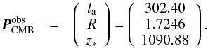 (32)The corresponding inverse covariance matrix can be written as
 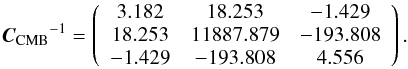 (33)The
  value of CMB is
 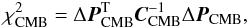 (34)where
  .
.
4. Methods and results
With the joint data, the total χ2 can be expressed as  (35)The model parameters can be determined by computing the χ2 distribution. First, we calculated the lowest value of the total χ2/ d.o.f. = 0.990 from simultaneous fitting. Then, we calculated the inverse covariance matrix to obtain the best-fit value 1σ uncertainty δ = − 0.022 ± 0.006,
  , w0 = − 1.210 ± 0.033, and w1 = 0.872 ± 0.072.
To obtain the contour plot, we marginalized two of the four parameters to derive a new χ2 function depending on the other two parameters, 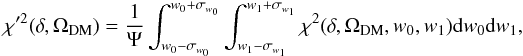 (36)where Ψ is the normalization factor to cause the χ′2 to have the same lowest value as χ2. Then we used χ′2 to derive the δ − ΩDM 2D marginalized regions with different colors that represent 1σ and 2σ regions. Figure 1 shows the δ − ΩDM contours with different data combinations: SNe (gray and light-gray contours), SNe + BAO (red and pink contours), SNe + CMB (blue and light-purple contours), CMB + BAO + H(z) (orange and yellow contours) and the full data-sets (black and cyan contours). This figure shows that the BAO data can set tight constraints on ΩDM, while CMB can set tighter constraints on δ and ΩDM. From Fig. 1, we find that the SNe data disagree with other data sets. This has been investigated by Nesseris & Perivolaropoulos (2005) and Wei (2010a).
 |
Fig. 1 δ − ΩDM contours with different data combinations: SNe (gray and light-gray contours), SNe + BAO (red and pink contours), SNe + CMB (blue and light-purple contours), CMB + BAO + H(z) (orange and yellow contours), and SNe + CMB + BAO + H(z) (black and cyan contours). The central regions and the vicinity regions represent the 1σ contours and 2σ contours. |
To test the reliability of our method, we also show the w0 − w1 contours from SNe+BAO+CMB without the coupling (δ = 0) with 1σ region in black contours and 2σ region in grey contours, which is presented in the left panel of Fig. 2. Our result is consistent with that of the WMAP team from comparing this figure with Fig. 10 of Hinshaw et al. (2013). The right panel of Fig. 2 shows the w0 − w1 contours with coupling. We show the δ − w0 and ΩDM − w1 contours in Fig. 3 and the δ − w1 and ΩDM − w0 contours in Fig. 4.
 |
Fig. 2 Black and gray regions are 1σ contours and 2σ contours. The left panel shows w0 vs. w1 without coupling, the right panel shows w0 vs. w1 with coupling in our model. |
 |
Fig. 3 Black and gray regions are 1σ contours and 2σ contours. The left panel shows δ vs. w0, the right panel shows ΩDM vs. w1. |
 |
Fig. 4 Black and gray regions are 1σ contours and 2σ contours. The left panel shows δ vs. w1, the right panel shows ΩDM vs. w0. |
From the best-fit parameters, the energy density evolution of DM and DE can be calculated. The ratio of DM density and DE density is ![Mathematical equation: \begin{eqnarray} \rho_{\rm DM}/\rho_{\rm DE}=\rho_{\rm DM}^{0}a^{-3+\delta}/\left(\rho_{\rm DE}^{\rm NI}(z)\left[1+\Theta(z,w_{0},w_{1},\delta)\right]\right).\label{DM/DE} \end{eqnarray}](/articles/aa/full_html/2014/04/aa22606-13/aa22606-13-eq122.png) (37)Figure 5 shows the evolution of ρDM/ρDE as a function of scale factor a with best-fit parameters. The gray region represents the 1σ uncertainty in this model, the black one represents the ΛCDM case. In our model, δ < 0 means that the energy is transferred from dark matter to dark energy, which is consisted with Dalal et al. (2001) and Guo et al. (2007). Nevertheless, the energy density proportion evolves slower than in ΛCDM case within 1σ uncertainties when a < 0.5, which means that our model can significantly help in reducing the coincidence problem.
(37)Figure 5 shows the evolution of ρDM/ρDE as a function of scale factor a with best-fit parameters. The gray region represents the 1σ uncertainty in this model, the black one represents the ΛCDM case. In our model, δ < 0 means that the energy is transferred from dark matter to dark energy, which is consisted with Dalal et al. (2001) and Guo et al. (2007). Nevertheless, the energy density proportion evolves slower than in ΛCDM case within 1σ uncertainties when a < 0.5, which means that our model can significantly help in reducing the coincidence problem.
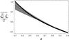 |
Fig. 5 Evolution of ρDM/ρDE as a function of scale factor a(z). The dashed line plots the interacting model with best-fit parameters, the gray region shows the 1σ uncertainties. The black region represents the ΛCDM with uncertainties. |
The evolution of DE density plays an important role in solving the coincidence problem. Using Eq. (9) we can compute the DE evolution, which is shown in Fig. 6. The gray region above the black line shows that the DE density decreases within 1σ when a < 0.5, which can slow down the evolution of ρDM/ρDE, resulting in a good solution to the coincidence problem. However, the DE density evolves quite quickly in the very early stage of the Universe when a < 0.3. The main reason is that DM mass transfer rate δ is assumed as a constant in our model.
 |
Fig. 6 Evolution of ρDE as a function of scale factor a(z). The dashed line plots the interacting model with best-fit parameters, the gray region shows the 1σ uncertainties. The black line represents the ΛCDM case. |
Our Universe is currently undergoing an accelerating expansion. But in the very early time, the Universe was decelerating. This means that the evolution of deceleration parameter q(z) is important, especially when q(ztr) = 0, ztr is the transition redshift. q(z) can be expressed as  (38)After substituting the best-fit parameters and their uncertainties in Eq. (38), we obtain ztr = 0.63 ± 0.07. This value is slightly higher than those of Wang & Dai (2006), Wang et al. (2007) and Abdel-Rahman & Riad (2007) in ΛCDM. The reason is the energy transfer from DM to DE in our model. The DM density decreases quicker than that in the ΛCDM, while the DE density decreases much quicker in early times. Therefore a higher transition redshfit is needed for DE to resist gravitation.
5. Conclusions and discussions
We used the Union 2.1 SNe Ia, CMB from WMAP 9 years, BAO observation data from 6dFGRS, SDSS DR7, BOSS DR9, WiggleZ, and the latest Hubble parameter data to test the phenomenological interacting dark sector scenario with a dynamic EoS wDE(z) = w0 + w1z/ (1 + z). We derived more stringent constraints on the phenomenological model parameters: δ = − 0.022 ± 0.006, , w0 = − 1.210 ± 0.033 and w1 = 0.872 ± 0.072 with  . From the contours using different data combinations in Fig. 1, we find that the SNe Ia data disagree with the combined CMB, BAO, and Hubble parameter data.
Our phenomenological scenario gives δ < 0 at 1σ confidence level, which is consistent with Dalal et al. (2001) and Guo et al. (2007). This indicates that the energy is transferred from dark matter to dark energy. But the evolution of ρDM/ρDE is slower than that in ΛCDM within 1σ uncertainties, because ρDE decreases with scale factor a. Therefore our model represents a good approach to solve the coincidence problem.
The DE density evolves quickly in the very early epoch of the Universe, which is shown in Fig. 6. The main reason is that the value of δ is assumed to be constant in our model. In reality, the DM mass transfer rate δ(a) needs to be varied. We also derived the transition redshit ztr = 0.63 ± 0.07 in this model. Because of the interaction between DE and DM, the DE density decreases very quickly in early times, therefore a higher transition redshift is needed to resist gravitation.
Acknowledgments
We thank the anonymous referee for helpful comments and suggestions that have helped us improve our manuscript. This work is supported by the National Basic Research Program of China (973 Program, grant 2014CB845800) and the National Natural Science Foundation of China (grants 11373022, 11103007, 11033002 and J1210039).
References
- Abdel-Rahman, A.-M. M., & Riad, I. F. 2007, AJ, 134, 1391 [NASA ADS] [CrossRef] [Google Scholar]
- Amendola, L. 2000, Phys. Rev. D, 62, 043511 [CrossRef] [Google Scholar]
- Amendola, L., Campos, G. C., & Rosenfeld, R. 2007, Phys. Rev. D, 75, 3506 [Google Scholar]
- Anderson, L., Aubourg, E., Bailey, S., et al. 2012, MNRAS, 427, 3435 [Google Scholar]
- Armendariz-Picon, C., Mukhanov, V., & Steinhardt, P. J. 2001, Phys. Rev. D, 63, 3510 [Google Scholar]
- Bertolami, O., Gil Pedro, F., & Le Delliou, M. 2007, Phys. Lett. B, 654, 165 [NASA ADS] [CrossRef] [Google Scholar]
- Beutler, F., Blake, C., Colless, M., et al. 2011, MNRAS, 416, 3017 [NASA ADS] [CrossRef] [Google Scholar]
- Blake, C., Brough, S., Colless, M., et al. 2012, MNRAS, 425, 405 [NASA ADS] [CrossRef] [Google Scholar]
- Busca, N. G., Delubac, T., Rich, J., et al. 2013, A&A, 552, A96 [NASA ADS] [CrossRef] [EDP Sciences] [Google Scholar]
- Cai, R.-G., & Su, Q. 2010, Phys. Rev. D, 81, 103514 [NASA ADS] [CrossRef] [Google Scholar]
- Caldwell, R. R. 2002, Phys. Lett. B, 545, 23 [NASA ADS] [CrossRef] [Google Scholar]
- Cao, S., Liang, N., & Zhu, Z.-H. 2011, Int. J. Mod. Phys. D, 22, 14 [Google Scholar]
- Chevallier, M., & Polarski, D. 2001, Int. J. Mod. Phys. D, 10, 213 [NASA ADS] [CrossRef] [Google Scholar]
- Chuang, C.-H., & Wang, Y. 2013, MNRAS, 1955 [Google Scholar]
- Cole, S., Percival, W. J., Peacock, J., et al. 2005, MNRAS, 362, 505 [NASA ADS] [CrossRef] [Google Scholar]
- Dalal, N., Abazajian, K., Jenkins, E., & Manohar, A. V. 2001, Phys. Rev. L, 87, 141302 [Google Scholar]
- Del Campo, S., Herrera, R., Olivares, G., & Pavón, D. 2006, Phys. Rev. D, 74, 023501 [NASA ADS] [CrossRef] [Google Scholar]
- Eisenstein, D. J., & Hu, W. 1998, ApJ, 496, 605 [NASA ADS] [CrossRef] [Google Scholar]
- Eisenstein, D. J., Zehavi, I., Hogg, D. W., et al. 2005, ApJ, 633, 560 [NASA ADS] [CrossRef] [Google Scholar]
- Farooq, O., & Ratra, B. 2013, ApJ, 766, L7 [NASA ADS] [CrossRef] [MathSciNet] [Google Scholar]
- Farrar, G. R., & Peebles, P. J. E. 2004, ApJ, 604, 1 [NASA ADS] [CrossRef] [Google Scholar]
- Feng, B., Wang, X., & Zhang, X. 2005, Phys. Lett. B, 607, 35 [NASA ADS] [CrossRef] [Google Scholar]
- Guo, Z.-K., Cai, R.-G., & Zhang, Y.-Z. 2005, JCAP, 5, 2 [Google Scholar]
- Guo, Z.-K., Ohta, N., & Tsujikawa, S. 2007, Phys. Rev. D, 76, 023508 [NASA ADS] [CrossRef] [Google Scholar]
- Hinshaw, G., Larson, D., Komatsu, E., et al. 2013, ApJS, 208, 19 [NASA ADS] [CrossRef] [Google Scholar]
- Hu, W., & Sugiyama, N. 1996, ApJ, 471, 542 [NASA ADS] [CrossRef] [Google Scholar]
- Linder, E. V. 2003, Phys. Rev. Lett., 90, 091301 [NASA ADS] [CrossRef] [PubMed] [Google Scholar]
- Majerotto, E., Sapone, D., & Amendola, L. 2004, unpublished [arXiv:astro-ph/0410543] [Google Scholar]
- Moresco, M., Cimatti, A., Jimenez, R., et al. 2012, JCAP, 8, 6 [Google Scholar]
- Nesseris, S., & Perivolaropoulos, L. 2005, Phys. Rev. D, 72, 123519 [NASA ADS] [CrossRef] [Google Scholar]
- Padmanabhan, N., Xu, X., Eisenstein, D. J., et al. 2012, MNRAS, 427, 2132 [NASA ADS] [CrossRef] [MathSciNet] [Google Scholar]
- Percival, W. J., Reid, B. A., Eisenstein, D. J., et al. 2010, MNRAS, 401, 2148 [NASA ADS] [CrossRef] [Google Scholar]
- Perlmutter, S., Aldering, G., Goldhaber, G., et al. 1999, ApJ, 517, 565 [NASA ADS] [CrossRef] [Google Scholar]
- Planck Collaboration XVI. 2014, A&A, in press, DOI: 10.1051/0004-6361/201321591 [Google Scholar]
- Ratra, B., & Peebles, P. J. E. 1988, Phys. Rev. D, 37, 3406 [NASA ADS] [CrossRef] [MathSciNet] [Google Scholar]
- Riess, A. G., Filippenko, A. V., Challis, P., et al. 1998, AJ, 116, 1009 [NASA ADS] [CrossRef] [Google Scholar]
- Riess, A. G., Macri, L., Casertano, S., et al. 2011, ApJ, 730, 119 [NASA ADS] [CrossRef] [Google Scholar]
- Rosenfeld, R. 2005, Phys. Lett. B, 624, 158 [NASA ADS] [CrossRef] [Google Scholar]
- Sadjadi, H. M., & Alimohammadi, M. 2006, Phys. Rev. D, 74, 103007 [NASA ADS] [CrossRef] [Google Scholar]
- Simon, J., Verde, L., & Jimenez, R. 2005, Phys. Rev. D, 71, 123001 [Google Scholar]
- Stern, D., Jimenez, R., Verde, L., Kamionkowski, M., & Stanford, S. A. 2010, JCAP, 2, 8 [Google Scholar]
- Suzuki, N., Rubin, D., Lidman, C., et al. 2012, ApJ, 746, 85 [NASA ADS] [CrossRef] [Google Scholar]
- Szydłowski, M., 2006, Phys. Lett. B, 632, 1 [NASA ADS] [CrossRef] [Google Scholar]
- Wang, F. Y. 2012, A&A, 543, A91 [NASA ADS] [CrossRef] [EDP Sciences] [Google Scholar]
- Wang, F. Y., & Dai, Z. G. 2006, MNRAS, 368, 371 [NASA ADS] [CrossRef] [Google Scholar]
- Wang, F. Y., Dai, Z. G., & Zhu, Z. H. 2007, ApJ, 667, 1 [NASA ADS] [CrossRef] [Google Scholar]
- Wei, H. 2010a, Phys. Lett. B, 687, 286 [NASA ADS] [CrossRef] [Google Scholar]
- Wei, H. 2010b, Phys. Lett. B, 691, 173 [NASA ADS] [CrossRef] [Google Scholar]
- Wei, H., & Cai, R.-G. 2006, Phys. Rev. D, 73, 083002 [NASA ADS] [CrossRef] [Google Scholar]
- Zhang, C., Zhang, H., Yuan, S., Zhang, T.-J., & Sun, Y.-C. 2012, ApJ, submitted [arXiv:1207.4541] [Google Scholar]
All Figures
|
Fig. 1 δ − ΩDM contours with different data combinations: SNe (gray and light-gray contours), SNe + BAO (red and pink contours), SNe + CMB (blue and light-purple contours), CMB + BAO + H(z) (orange and yellow contours), and SNe + CMB + BAO + H(z) (black and cyan contours). The central regions and the vicinity regions represent the 1σ contours and 2σ contours. |
| In the text | |
|
Fig. 2 Black and gray regions are 1σ contours and 2σ contours. The left panel shows w0 vs. w1 without coupling, the right panel shows w0 vs. w1 with coupling in our model. |
| In the text | |
|
Fig. 3 Black and gray regions are 1σ contours and 2σ contours. The left panel shows δ vs. w0, the right panel shows ΩDM vs. w1. |
| In the text | |
|
Fig. 4 Black and gray regions are 1σ contours and 2σ contours. The left panel shows δ vs. w1, the right panel shows ΩDM vs. w0. |
| In the text | |
|
Fig. 5 Evolution of ρDM/ρDE as a function of scale factor a(z). The dashed line plots the interacting model with best-fit parameters, the gray region shows the 1σ uncertainties. The black region represents the ΛCDM with uncertainties. |
| In the text | |
|
Fig. 6 Evolution of ρDE as a function of scale factor a(z). The dashed line plots the interacting model with best-fit parameters, the gray region shows the 1σ uncertainties. The black line represents the ΛCDM case. |
| In the text | |
Current usage metrics show cumulative count of Article Views (full-text article views including HTML views, PDF and ePub downloads, according to the available data) and Abstracts Views on Vision4Press platform.
Data correspond to usage on the plateform after 2015. The current usage metrics is available 48-96 hours after online publication and is updated daily on week days.
Initial download of the metrics may take a while.