| Issue |
A&A
Volume 564, April 2014
|
|
|---|---|---|
| Article Number | A2 | |
| Number of page(s) | 11 | |
| Section | The Sun | |
| DOI | https://doi.org/10.1051/0004-6361/201322315 | |
| Published online | 26 March 2014 | |
Magnetic flux concentrations in a polytropic atmosphere
1
Nordita, KTH Royal Institute of Technology and Stockholm
University, Roslagstullsbacken
23, 10691
Stockholm,
Sweden
e-mail:
This email address is being protected from spambots. You need JavaScript enabled to view it.
2
Department of Astronomy, AlbaNova University Center, Stockholm
University, 10691
Stockholm,
Sweden
3
Department of Mechanical Engineering, Ben-Gurion University of the
Negev, POB 653,
84105
Beer-Sheva,
Israel
4
Department of Radio Physics, N. I. Lobachevsky State University of
Nizhny Novgorod, 603950
Nizhnü Novgorod,
Russia
Received:
18
July
2013
Accepted:
23
January
2014
Abstract
Context. Strongly stratified hydromagnetic turbulence has recently been identified as a candidate for explaining the spontaneous formation of magnetic flux concentrations by the negative effective magnetic pressure instability (NEMPI). Much of this work has been done for isothermal layers, in which the density scale height is constant throughout.
Aims. We now want to know whether earlier conclusions regarding the size of magnetic structures and their growth rates carry over to the case of polytropic layers, in which the scale height decreases sharply as one approaches the surface.
Methods. To allow for a continuous transition from isothermal to polytropic layers, we employ a generalization of the exponential function known as the q-exponential. This implies that the top of the polytropic layer shifts with changing polytropic index such that the scale height is always the same at some reference height. We used both mean-field simulations (MFS) and direct numerical simulations (DNS) of forced stratified turbulence to determine the resulting flux concentrations in polytropic layers. Cases of both horizontal and vertical applied magnetic fields were considered.
Results. Magnetic structures begin to form at a depth where the magnetic field strength is a small fraction of the local equipartition field strength with respect to the turbulent kinetic energy. Unlike the isothermal case where stronger fields can give rise to magnetic flux concentrations at larger depths, in the polytropic case the growth rate of NEMPI decreases for structures deeper down. Moreover, the structures that form higher up have a smaller horizontal scale of about four times their local depth. For vertical fields, magnetic structures of super-equipartition strengths are formed, because such fields survive downward advection that causes NEMPI with horizontal magnetic fields to reach premature nonlinear saturation by what is called the “potato-sack” effect. The horizontal cross-section of such structures found in DNS is approximately circular, which is reproduced with MFS of NEMPI using a vertical magnetic field.
Conclusions. Results based on isothermal models can be applied locally to polytropic layers. For vertical fields, magnetic flux concentrations of super-equipartition strengths form, which supports suggestions that sunspot formation might be a shallow phenomenon.
Key words: magnetohydrodynamics (MHD) / hydrodynamics / turbulence / Sun: dynamo
© ESO, 2014
1. Introduction
In a turbulent medium, the turbulent pressure can lead to dynamically important effects. In particular, a stratified layer can attain a density distribution that is significantly altered compared to the nonturbulent case. In addition, magnetic fields can change the situation further, because it can locally suppress the turbulence and thus reduce the total turbulent pressure (the sum of hydrodynamic and magnetic turbulent contributions). On length scales encompassing many turbulent eddies, this total turbulent pressure reduction must be compensated for by additional gas pressure, which can lead to a density enhancement and thus to horizontal magnetic structures that become heavier than the surroundings and sink (Brandenburg et al. 2011). This is quite the contrary of magnetic buoyancy, which is still expected to operate on the smaller scale of magnetic flux tubes and in the absence of turbulence. Both effects can lead to instability: the latter is the magnetic buoyancy or interchange instability (Newcomb 1961; Parker 1966), and the former is now often referred to as negative effective magnetic pressure instability (NEMPI), which has been studied at the level of mean-field theory for the past two decades (Kleeorin et al. 1989, 1990, 1993, 1996; Kleeorin & Rogachevskii 1994; Rogachevskii & Kleeorin 2007). These are instabilities of a stratified continuous magnetic field, while the usual magnetic buoyancy instability requires nonuniform and initially separated horizontal magnetic flux tubes (Parker 1955; Spruit 1981; Schüssler et al. 1994).
Unlike the magnetic buoyancy instability, NEMPI occurs at the expense of turbulent energy rather than the energy of the gravitational field. The latter is the energy source of the magnetic buoyancy or interchange instability. NEMPI is caused by a negative turbulent contribution to the effective mean magnetic pressure (the sum of nonturbulent and turbulent contributions). For large Reynolds numbers, this turbulent contribution to the effective magnetic pressure is larger than the nonturbulent one. This results in the excitation of NEMPI and the formation of large-scale magnetic structures – even from an originally uniform mean magnetic field.
Direct numerical simulations (DNS) have recently demonstrated the operation of NEMPI in isothermally stratified layers (Brandenburg et al. 2011; Kemel et al. 2012b). This is a particularly simple case in that the density scale height is constant; i.e., the computational burden of covering large density variation is distributed over the depth of the entire layer. In spite of this simplification, it has been argued that NEMPI is important for explaining prominent features in the manifestation of solar surface activity. In particular, it has been associated with the formation of active regions (Kemel et al. 2013; Warnecke et al. 2013) and sunspots (Brandenburg et al. 2013, 2014). However, it is now important to examine the validity of conclusions based on such simplifications using more realistic models. In this paper, we therefore now consider a polytropic stratification, for which the density scale height is smallest in the upper layers, and the density variation therefore greatest.
NEMPI is a large-scale instability that can be excited in stratified small-scale
turbulence. This requires (i) sufficient scale separation in the sense that the maximum
scale of turbulent motions, ℓ, must be much smaller than the scale of the system,
L; and (ii)
strong density stratification such that the density scale height Hρ is much smaller than
L; i.e.,
 (1)However,
both the size of turbulent motions and the typical size of perturbations due to NEMPI can be
related to the density scale height. Furthermore, earlier work of Kemel et al. (2013) using isothermal layers shows that the scale of
perturbations due to NEMPI exceeds the typical density scale height. Unlike the isothermal
case, in which the scale height is constant, it decreases rapidly with height in a
polytropic layer. It is then unclear how such structures could fit into the narrow space
left by the stratification and whether the scalings derived for the isothermal case can
still be applied locally to polytropic layers.
(1)However,
both the size of turbulent motions and the typical size of perturbations due to NEMPI can be
related to the density scale height. Furthermore, earlier work of Kemel et al. (2013) using isothermal layers shows that the scale of
perturbations due to NEMPI exceeds the typical density scale height. Unlike the isothermal
case, in which the scale height is constant, it decreases rapidly with height in a
polytropic layer. It is then unclear how such structures could fit into the narrow space
left by the stratification and whether the scalings derived for the isothermal case can
still be applied locally to polytropic layers.
NEMPI has already been studied previously for polytropic layers in mean-field simulations (MFS; Brandenburg et al. 2010; Käpylä et al. 2012; Jabbari et al. 2013), but no systematic comparison has been made with NEMPI in isothermal or in polytropic layers with different values of the polytropic index. This will be done in the present paper, both in MFS and DNS. Those two complementary types of simulations have proved to be a good tool for understanding the underlying physics of NEMPI. An example are the studies of the effects of rotation on NEMPI (Losada et al. 2012, 2013), where MFS have been able to give quantitatively useful predictions before corresponding DNS were able to confirm the resulting dependence.
2. Polytropic stratification
We discuss here the equation for the vertical profile of the fluid density in a polytropic
layer. In a Cartesian plane-parallel layer with polytropic stratification, the temperature
gradient is constant, so the temperature goes linearly to zero at z∞. The
temperature, T,
is proportional to the square of the sound speed,  , and thus also to
the density scale height Hρ(z),
which is given by
, and thus also to
the density scale height Hρ(z),
which is given by  for an
isentropic stratification, where g is the acceleration due to the
gravity. For a perfect gas, the density ρ is proportional to Tn, and the pressure
p is
proportional to Tn+1, such that
p/ρ is
proportional to T, where n is the polytropic index. Furthermore, we have
p(z) ∝ ρ(z)Γ,
where Γ = (n + 1)/n is
another useful coefficient.
for an
isentropic stratification, where g is the acceleration due to the
gravity. For a perfect gas, the density ρ is proportional to Tn, and the pressure
p is
proportional to Tn+1, such that
p/ρ is
proportional to T, where n is the polytropic index. Furthermore, we have
p(z) ∝ ρ(z)Γ,
where Γ = (n + 1)/n is
another useful coefficient.
For a perfect gas, the specific entropy can be defined (up to an additive constant) as
s = cvln(p/ργ),
where γ = cp/cv
is the ratio of specific heats at constant pressure and constant density, respectively. For
a polytropic stratification, we have  (2)so s is constant when
Γ = γ, which
is the case for an isentropic stratification. In the following, we make this assumption and
specify from now only the value of γ. For a monatomic gas, we have γ = 5/3,
which is relevant for the Sun, while for a diatomic molecular gas, we have γ = 7/5,
which is relevant for air. In those cases, a stratification with Γ = γ can be motivated by
assuming perfect mixing across the layer. The isothermal case with γ = 1 can be motivated by
assuming rapid heating/cooling to a constant temperature.
(2)so s is constant when
Γ = γ, which
is the case for an isentropic stratification. In the following, we make this assumption and
specify from now only the value of γ. For a monatomic gas, we have γ = 5/3,
which is relevant for the Sun, while for a diatomic molecular gas, we have γ = 7/5,
which is relevant for air. In those cases, a stratification with Γ = γ can be motivated by
assuming perfect mixing across the layer. The isothermal case with γ = 1 can be motivated by
assuming rapid heating/cooling to a constant temperature.
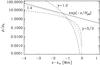 |
Fig. 1 Isothermal and polytropic relations for different values of γ when calculated using the conventional formula ρ ∝ (z∞ − z)n with n = 1/(γ − 1). |
Our aim is to study the change in the properties of NEMPI in a continuous fashion as we go
from an isothermally stratified layer to a polytropic one. In the latter case, the fluid
density varies in a power law fashion, ρ ∝ (z∞ − z)n,
while in the former, it varies exponentially, ρ ∝ exp(z∞ − z).
This is shown in Fig. 1 where we compare the
exponential isothermal atmosphere with a family of polytropic atmospheres with
γ = 1.2, 1.4,
and 5/3. Clearly, there is no continuous connection between the isothermal case and the
polytropic one in the limit γ → 1. This cannot be fixed by rescaling the isothermal
density stratification, because in Fig. 1 its values
would still lie closer to 5/3 than to 1.4 or 1.2. Another problem with this description is
that for polytropic solutions the density is always zero at z = z∞, but finite in the
isothermal case. These different behaviors between isothermal and polytropic atmospheres can
be unified by using the generalized exponential function known as the “q-exponential” (see, e.g.,
Yamano 2002), which is defined as ![Mathematical equation: \begin{equation} e_q(x)=\left[1+(1-q)x\right]^{1/(1-q)}, \label{EQ} \end{equation}](/articles/aa/full_html/2014/04/aa22315-13/aa22315-13-eq35.png) (3)where the parameter
q is related
to γ via
q = 2 − γ. This generalization of the
usual exponential function was originally introduced by Tsallis (1988) in connection with a possible generalization of the Boltzmann-Gibbs
statistics. Its usefulness in connection with stellar polytropes has been employed by Plastino & Plastino (1993). Thus, the density
stratification is given by
(3)where the parameter
q is related
to γ via
q = 2 − γ. This generalization of the
usual exponential function was originally introduced by Tsallis (1988) in connection with a possible generalization of the Boltzmann-Gibbs
statistics. Its usefulness in connection with stellar polytropes has been employed by Plastino & Plastino (1993). Thus, the density
stratification is given by ![Mathematical equation: \begin{equation} \frac{\rho}{\rho_0}=\left[1+(\gamma-1)\left( -{z\over H_{\rho0}}\right)\right ]^{1/(\gamma\,-\,1)} =\left(1-{z\over nH_{\rho0}}\right)^n,\quad \label{rho_gen} \end{equation}](/articles/aa/full_html/2014/04/aa22315-13/aa22315-13-eq37.png) (4)which
reduces to ρ/ρ0 = exp(−z/Hρ0)
for isothermal stratification with γ → 1 and n → ∞. The density scale height is then given by
(4)which
reduces to ρ/ρ0 = exp(−z/Hρ0)
for isothermal stratification with γ → 1 and n → ∞. The density scale height is then given by
 (5)In the following, we
measure lengths in units of Hρ0 = Hρ(0).
(5)In the following, we
measure lengths in units of Hρ0 = Hρ(0).
In Fig. 2 we show the dependencies of ρ(z) and Hρ given by Eqs. (4) and (5) for different values of γ. Compared with Fig. 1, where z∞ is held fixed, in Fig. 2 it is equal to z∞ = nHρ0 = Hρ0/(γ − 1). The total density contrast is roughly the same in all four cases for different γ, but for increasing values of γ, the vertical density gradient becomes progressively stronger in the upper layers.
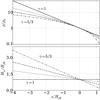 |
Fig. 2 Polytropes (Eq. (4)) with γ = 1 (solid line), 1.2 (dash-dotted), 1.4 (dotted), and 5/3 (dashed) and density scale height (Eq. (5)) for −4 ≤ −z/Hρ0 ≤ 1.2. The total density contrast is similar for γ = 1 and 5/3. |
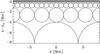 |
Fig. 3 Sketch showing the expected size distribution of the nearly circular NEMPI eigenfunction structures at different heights. |
Assuming that the radius R of the resulting structures is proportional to
Hρ, we sketch in Fig. 3 a situation in which R is half the depth. With
ρ ∝ (z∞ − z)n,
the density scale height is Hρ(z) = (z∞ − z)/n.
Thus, Fig. 3 applies to a case in which R = (z∞ − z)/2 = (n/2) Hρ(z).
The solar convection zone is nearly isentropic and well described by n = 3/2.
This means that the structures of Fig. 3 have
R = (3/4) Hρ(z).
The results of Kemel et al. (2013) and Brandenburg et al. (2014) suggest that the horizontal
wavenumber of structures, k⊥, formed by NEMPI, is less than or about
 ,
so their horizontal wavelength is ≲2πHρ.
One wavelength corresponds to the distance between two nodes, i.e., the distance between two
spheres, which is 4 R. Thus, in the isothermal case we have
R/Hρ = 2π/4 ≈ 1.5,
which implies that such a structure would not fit into the isentropic atmosphere described
above. This provides an additional motivation for our present work.
,
so their horizontal wavelength is ≲2πHρ.
One wavelength corresponds to the distance between two nodes, i.e., the distance between two
spheres, which is 4 R. Thus, in the isothermal case we have
R/Hρ = 2π/4 ≈ 1.5,
which implies that such a structure would not fit into the isentropic atmosphere described
above. This provides an additional motivation for our present work.
3. DNS study
In this section we study NEMPI in DNS for the polytropic layer. Corresponding MFS are presented in Sect. 4.
3.1. The model
We solve the equations for the magnetic vector potential A, the velocity U, and the density ρ, in the form
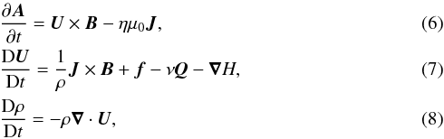 where
D/Dt = ∂/∂t + U·∇
is the advective derivative with respect to the actual (turbulent) flow, B = B0 + ∇ × A
is the magnetic field, B0 the imposed uniform
field, J = ∇ × B/μ0
the current density, μ0 the vacuum permeability,
H = h + Φ the reduced enthalpy,
h = cpT
the enthalpy, Φ is the
gravitational potential,
where
D/Dt = ∂/∂t + U·∇
is the advective derivative with respect to the actual (turbulent) flow, B = B0 + ∇ × A
is the magnetic field, B0 the imposed uniform
field, J = ∇ × B/μ0
the current density, μ0 the vacuum permeability,
H = h + Φ the reduced enthalpy,
h = cpT
the enthalpy, Φ is the
gravitational potential, 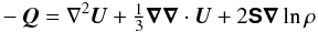 (9)is
a term appearing in the viscous force −νQ, S is the traceless
rate-of-strain tensor with components
(9)is
a term appearing in the viscous force −νQ, S is the traceless
rate-of-strain tensor with components
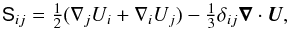 (10)ν is the kinematic
viscosity, and η is the magnetic diffusion coefficient caused by
electrical conductivity of the fluid. As in Losada et al.
(2012), z corresponds to radius, x to colatitude, and
y to
azimuth. The forcing function f consists of random, white-in-time,
plane, nonpolarized waves with a certain average wavenumber kf.
(10)ν is the kinematic
viscosity, and η is the magnetic diffusion coefficient caused by
electrical conductivity of the fluid. As in Losada et al.
(2012), z corresponds to radius, x to colatitude, and
y to
azimuth. The forcing function f consists of random, white-in-time,
plane, nonpolarized waves with a certain average wavenumber kf.
3.2. Boundary conditions and parameters
In the DNS we use stress-free boundary conditions for the velocity at the top and bottom; i.e., ∇zUx = ∇zUy = Uz = 0. For the magnetic field we use either perfect conductor boundary conditions, Ax = Ay = ∇zAz = 0, or vertical field conditions, ∇zAx = ∇zAy = Az = 0, again at both the top and bottom. All variables are assumed periodic in the x and y directions.
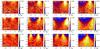 |
Fig. 4 Snapshots of |
The turbulent rms velocity is approximately independent of z with
 . The
gravitational acceleration g = (0,0, −g)
is chosen such that k1Hρ0 = 1,
where k1 = 2π/L
and L is the
size of the domain. With one exception (Sect. 3.5),
we always use the value kf/k1 = 30
for the scale separation ratio. For B0 we choose either a
horizontal field pointing in the y direction or a vertical one pointing in the
z
direction. The latter case, B0 = (0,0,B0),
is usually combined with the use of the vertical field boundary condition, while the
former one, B0 = (0,B0,0),
is combined with using perfect conductor boundary conditions. The strength of the imposed
field is expressed in terms of Beq0 = Beq(z = 0),
which is the equipartition field strength at z = 0. Here, the equipartition field
. The
gravitational acceleration g = (0,0, −g)
is chosen such that k1Hρ0 = 1,
where k1 = 2π/L
and L is the
size of the domain. With one exception (Sect. 3.5),
we always use the value kf/k1 = 30
for the scale separation ratio. For B0 we choose either a
horizontal field pointing in the y direction or a vertical one pointing in the
z
direction. The latter case, B0 = (0,0,B0),
is usually combined with the use of the vertical field boundary condition, while the
former one, B0 = (0,B0,0),
is combined with using perfect conductor boundary conditions. The strength of the imposed
field is expressed in terms of Beq0 = Beq(z = 0),
which is the equipartition field strength at z = 0. Here, the equipartition field
 . The imposed field
is normalized by Beq0 and denoted as β0 = B0/Beq0,
while
. The imposed field
is normalized by Beq0 and denoted as β0 = B0/Beq0,
while  is the modulus
of the normalized mean magnetic field. Time is expressed in terms of the
turbulent-diffusive time,
is the modulus
of the normalized mean magnetic field. Time is expressed in terms of the
turbulent-diffusive time,  , where
ηt0 = urms/3kf
(Sur et al. 2008) is an estimate for the
turbulent magnetic diffusivity used in the DNS.
, where
ηt0 = urms/3kf
(Sur et al. 2008) is an estimate for the
turbulent magnetic diffusivity used in the DNS.
Our values of ν and η are characterized by specifying the kinetic and
magnetic Reynolds numbers,  (11)In
most of this paper (except in Sect. 3.5) we use
Re = 36 and Rm = 18, which
are also the values used by Kemel et al. (2013).
(11)In
most of this paper (except in Sect. 3.5) we use
Re = 36 and Rm = 18, which
are also the values used by Kemel et al. (2013).
The DNS are performed with the Pencil Code, http://pencil-code.googlecode.com, which uses sixth-order explicit finite differences in space and a third-order accurate time stepping method. We use a numerical resolution of 2563 mesh points.
3.3. Horizontal fields
We focus on the case γ = 5/3 and show in Fig. 4 visualizations of
 at different
instants for three values of the imposed horizontal magnetic field strength. For
β0 = 0.02, a magnetic structure is clearly
visible at t/τtd = 1.43,
while for β0 = 0.05 structures are already fully
developed at t/τtd = 0.42.
In that case (β0 = 0.05), at early times
(t/τtd = 0.42),
there are two structures, which then begin to merge at t/τtd = 1.38.
The growth rate of the magnetic structure is found to be
at different
instants for three values of the imposed horizontal magnetic field strength. For
β0 = 0.02, a magnetic structure is clearly
visible at t/τtd = 1.43,
while for β0 = 0.05 structures are already fully
developed at t/τtd = 0.42.
In that case (β0 = 0.05), at early times
(t/τtd = 0.42),
there are two structures, which then begin to merge at t/τtd = 1.38.
The growth rate of the magnetic structure is found to be
 for the runs
shown in Fig. 4. This is less than the value of
for the runs
shown in Fig. 4. This is less than the value of
 found earlier
for the isothermal case (Kemel et al. 2012b).
found earlier
for the isothermal case (Kemel et al. 2012b).
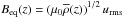
 |
Fig. 5 Snapshots from DNS showing |
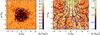 |
Fig. 6 Cuts of Bz/Beq(z) in (a) the xy plane at the top boundary (z/Hρ0 = 1.2) and (b) the xz plane through the middle of the spot at y = 0 for γ = 5/3 and β0 = 0.05. In the xz cut, we also show magnetic field lines and flow vectors obtained by numerically averaging in azimuth around the spot axis. |
For γ = 5/3 and β0 ≤ 0.02, the magnetic structures become smaller (k⊥Hρ0 = 2) near the surface. In the nonlinear regime, i.e., at late times, the structures move downward due to the so-called “potato-sack” effect, which was first seen in MFS (Brandenburg et al. 2010) and later confirmed in DNS (Brandenburg et al. 2011). The magnetic structures sink in the nonlinear stage of NEMPI, because an increase in the mean magnetic field inside the horizontal magnetic flux tube increases the absolute value of the effective magnetic pressure. On the other hand, a decrease in the negative effective magnetic pressure is balanced out by increased gas pressure, which in turn leads to higher density, so the magnetic structures become heavier than the surroundings and sink. This potato-sack effect has been clearly observed in the present DNS with the polytropic layer (see the right column in Fig. 4).
3.4. Vertical fields
Recent DNS using isothermal layers have shown that strong circular flux concentrations
can be produced in the case of a vertical magnetic field (Brandenburg et al. 2013, 2014). This is
also observed in the present study of a polytropic layer; see Fig. 5, where we show the evolution of
 on the periphery
of the computational domain for γ = 5/3 and β0 = 0.05 at
different times. A difference to the DNS for γ = 1 (Brandenburg
et al. 2013) seems to be that for γ = 5/3 the magnetic structures
are shallower than for γ = 1; see Fig. 6, where we show xy and xz slices of Bz through the spot.
Owing to periodicity in the xy plane, we have shifted the location of the spot to
x = y = 0. We note also that the
field lines of the averaged magnetic field show a structure rather similar to the one
found in MFS of Brandenburg et al. (2014). The
origin of circular structures is associated with a cylindrical symmetry for the vertical
magnetic field. The growth rate of the magnetic field in the spot is found to be
on the periphery
of the computational domain for γ = 5/3 and β0 = 0.05 at
different times. A difference to the DNS for γ = 1 (Brandenburg
et al. 2013) seems to be that for γ = 5/3 the magnetic structures
are shallower than for γ = 1; see Fig. 6, where we show xy and xz slices of Bz through the spot.
Owing to periodicity in the xy plane, we have shifted the location of the spot to
x = y = 0. We note also that the
field lines of the averaged magnetic field show a structure rather similar to the one
found in MFS of Brandenburg et al. (2014). The
origin of circular structures is associated with a cylindrical symmetry for the vertical
magnetic field. The growth rate of the magnetic field in the spot is found to be
 , which is
similar to the value of 1.3 found earlier for the isothermal case (Brandenburg et al. 2013).
, which is
similar to the value of 1.3 found earlier for the isothermal case (Brandenburg et al. 2013).
3.5. Effective magnetic pressure
As pointed out in Sect. 1, the main reason for the formation of strongly inhomogeneous large-scale magnetic structures is the negative contribution of turbulence to the large-scale magnetic pressure, so that the effective magnetic pressure (the sum of turbulent and nonturbulent contributions) can be negative at high magnetic Reynolds numbers. The effective magnetic pressure has been determined from DNS for isothermally stratified forced turbulence (Brandenburg et al. 2010, 2012) and for turbulent convection (Käpylä et al. 2012). To see whether the nature of polytropic stratification has any influence on the effective magnetic pressure, we use DNS.
We first explain the essence of the effect of turbulence on the effective magnetic
pressure. We consider the momentum equation in the form
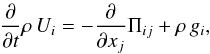 (12)where
 (13)is
the momentum stress tensor and δij the Kronecker
tensor.
(13)is
the momentum stress tensor and δij the Kronecker
tensor.
Ignoring correlations between velocity and density fluctuations for low-Mach number
turbulence, the averaged momentum equation is
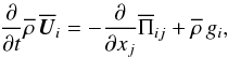 (14)where
an overbar means xy averaging,
(14)where
an overbar means xy averaging,  is the mean momentum stress tensor, split into contributions resulting from the mean field
(indicated by superscript m) and the fluctuating field (indicated by superscript f). The
tensor
is the mean momentum stress tensor, split into contributions resulting from the mean field
(indicated by superscript m) and the fluctuating field (indicated by superscript f). The
tensor  has the same form as Eq. (13), but all
quantities have now attained an overbar; i.e.,
has the same form as Eq. (13), but all
quantities have now attained an overbar; i.e.,
 (15)The
contributions,
(15)The
contributions,  ,
which result from the fluctuations
,
which result from the fluctuations  and
and  of
velocity and magnetic fields, respectively, are determined by the sum of the Reynolds and
Maxwell stress tensors:
of
velocity and magnetic fields, respectively, are determined by the sum of the Reynolds and
Maxwell stress tensors: 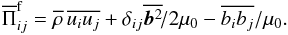 (16)This
contribution, together with the contribution from the mean field,
,
comprises the total mean momentum tensor. The contribution from the fluctuating fields is
split into a contribution that is independent of the mean magnetic field
(16)This
contribution, together with the contribution from the mean field,
,
comprises the total mean momentum tensor. The contribution from the fluctuating fields is
split into a contribution that is independent of the mean magnetic field
 (which determines the turbulent viscosity and background turbulent pressure) and a
contribution that depends on the mean magnetic field
(which determines the turbulent viscosity and background turbulent pressure) and a
contribution that depends on the mean magnetic field
 .
The difference between the two,
.
The difference between the two,  ,
is caused by the mean magnetic field and is parameterized in the form
,
is caused by the mean magnetic field and is parameterized in the form  (17)where
the coefficient qp represents the isotropic turbulence
contribution to the mean magnetic pressure, the coefficient qs represents
the turbulence contribution to the mean magnetic tension, while the coefficient
qg is the anisotropic turbulence
contribution to the mean magnetic pressure, and it characterizes the effect of vertical
variations of the magnetic field caused by the vertical magnetic pressure gradient. Here,
ĝi is the unit vector
in the direction of the gravity field (in the vertical direction). We consider cases with
horizontal and vertical mean magnetic fields separately. Analytically, the coefficients
qp, qg, and qs have been
obtained using both the spectral τ approach (Rogachevskii & Kleeorin 2007) and the renormalization approach (Kleeorin & Rogachevskii 1994). The form of Eq.
(17) is also obtained using simple
symmetry arguments; e.g., for a horizontal field, the linear combination of three
independent true tensors, δij,ĝiĝj
and
(17)where
the coefficient qp represents the isotropic turbulence
contribution to the mean magnetic pressure, the coefficient qs represents
the turbulence contribution to the mean magnetic tension, while the coefficient
qg is the anisotropic turbulence
contribution to the mean magnetic pressure, and it characterizes the effect of vertical
variations of the magnetic field caused by the vertical magnetic pressure gradient. Here,
ĝi is the unit vector
in the direction of the gravity field (in the vertical direction). We consider cases with
horizontal and vertical mean magnetic fields separately. Analytically, the coefficients
qp, qg, and qs have been
obtained using both the spectral τ approach (Rogachevskii & Kleeorin 2007) and the renormalization approach (Kleeorin & Rogachevskii 1994). The form of Eq.
(17) is also obtained using simple
symmetry arguments; e.g., for a horizontal field, the linear combination of three
independent true tensors, δij,ĝiĝj
and  , yields Eq.
(17), while for the vertical field, the
linear combination of only two independent true tensors, δij and
.
, yields Eq.
(17), while for the vertical field, the
linear combination of only two independent true tensors, δij and
.
Previous DNS studies (Brandenburg et al. 2012) have
shown that qs and qg are
negligible for forced turbulence. To avoid the formation of magnetic structures in the
nonlinear stage of NEMPI, which would modify our results, we use here a lower scale
separation ratio, kf/k1 = 5,
keeping k1Hρ = 1,
and using Re = 140 and
Rm = 70, as in Brandenburg et al. (2012). To determine qp(β), it is sufficient
to measure the three diagonal components of
both with and without an imposed magnetic field using
 .
.
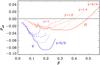 |
Fig. 7 Effective magnetic pressure obtained from DNS in a polytropic layer with different γ for horizontal (H, red curves) and vertical (V, blue curves) mean magnetic fields. |
In Fig. 7 we present the results for forced
turbulence in the polytropic layer with different γ for horizontal and
vertical mean magnetic fields. It turns out that the normalized effective magnetic
pressure, 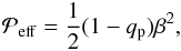 (18)has
a minimum value
(18)has
a minimum value  at βmin. Following Kemel et al. (2012a), the function qp(β) is approximated by:
 (19)where
qp0, βp, and
(19)where
qp0, βp, and
 are
constants. This equation can be understood as a quenching formula for the effective
magnetic pressure; see Jabbari et al. (2013). The
coefficients βp and β⋆ are related to
at βmin via (Kemel et al. 2012a)
are
constants. This equation can be understood as a quenching formula for the effective
magnetic pressure; see Jabbari et al. (2013). The
coefficients βp and β⋆ are related to
at βmin via (Kemel et al. 2012a)  (20)In Fig. 8 we show these fitting parameters for the function
qp(β) for polytropic
layer with different γ for horizontal and vertical mean magnetic fields.
The effects of negative effective magnetic pressure are generally stronger for vertical
magnetic fields (qp0 is larger and βp smaller) than
for horizontal ones (qp0 is smaller and βp larger), but
the values are
similar in both cases, and increasing from 0.35 (for γ = 1) to 0.6 (for
γ = 5/3); see Fig. 8.
(20)In Fig. 8 we show these fitting parameters for the function
qp(β) for polytropic
layer with different γ for horizontal and vertical mean magnetic fields.
The effects of negative effective magnetic pressure are generally stronger for vertical
magnetic fields (qp0 is larger and βp smaller) than
for horizontal ones (qp0 is smaller and βp larger), but
the values are
similar in both cases, and increasing from 0.35 (for γ = 1) to 0.6 (for
γ = 5/3); see Fig. 8.
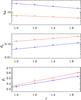 |
Fig. 8 Parameters qp0, βp, and β⋆ for the function qp(β) (see Eq. (19)) versus γ for horizontal (red line) and vertical (blue line) mean magnetic fields. |
4. Mean-field study
We now consider two sets of parameters that we refer to as Model I (with qp0 = 32 and βp = 0.058 corresponding to β⋆ = 0.33) and Model II (qp0 = 9 and βp = 0.21 corresponding to β⋆ = 0.63). These cases are representative of the strong (large β⋆) and weak (small β⋆) effects of NEMPI. Following earlier studies (Brandenburg et al. 2012), we find qs to be compatible with zero. We thus neglect this coefficient in the following.
4.1. Governing parameters and estimates
The purpose of this section is to summarize the findings for the isothermal case in MFS.
One of the key results is the prediction of the growth rate of NEMPI. The work of Kemel et al. (2013) showed that in the ideal case (no
turbulent diffusion), the growth rate λ is approximated well by  (21)However, turbulent
magnetic diffusion, ηt, can clearly not be neglected and is
chiefly responsible for shutting off NEMPI if the turbulent eddies are too big and
ηt too large. This was demonstrated in
Fig. 17 of Brandenburg et al. (2012). A heuristic
ansatz, which is motivated by similar circumstances in mean-field dynamo theory (Krause & Rädler 1980), is to add a term
−ηtk2 to
the righthand side of Eq. (21), where
k is the
wavenumber of NEMPI.
(21)However, turbulent
magnetic diffusion, ηt, can clearly not be neglected and is
chiefly responsible for shutting off NEMPI if the turbulent eddies are too big and
ηt too large. This was demonstrated in
Fig. 17 of Brandenburg et al. (2012). A heuristic
ansatz, which is motivated by similar circumstances in mean-field dynamo theory (Krause & Rädler 1980), is to add a term
−ηtk2 to
the righthand side of Eq. (21), where
k is the
wavenumber of NEMPI.
To specify the expression for λ, we normalize the wavenumber of the perturbations
by the inverse density scale height and denote this by κ ≡ kHρ.
The wavenumber of the energy-carrying turbulent eddies kf is in
nondimensional form κf ≡ kfHρ,
and the normalized horizontal wavenumber of the resulting magnetic structures is referred
to as κ⊥ = k⊥Hρ.
For NEMPI, these values have been estimated to be κ⊥ = 0.8–1.0,
and can even be smaller for vertical magnetic fields (Brandenburg et al. 2014). Using an approximate aspect ratio of unity for
magnetic structures, we have  –1.4.
In stellar mixing length theory (Vitense 1953), the
mixing length is ℓf = αmixHρ,
where αmix ≈ 1.6 is a nondimensional mixing
length parameter. Since kf = 2π/ℓf,
we arrive at the following estimate: κf = 2πγ/αmix ≈ 6.5.
[Owing to a confusion between pressure and density scale heights, this value was
underestimated by Kemel et al. (2013) to be
2.4, although an independent
calculation of this value from turbulent convection simulations would still be useful.]
Using ηt ≈ urms/3kf,
the turbulent magnetic diffusive rate for an isothermal atmosphere is given by
–1.4.
In stellar mixing length theory (Vitense 1953), the
mixing length is ℓf = αmixHρ,
where αmix ≈ 1.6 is a nondimensional mixing
length parameter. Since kf = 2π/ℓf,
we arrive at the following estimate: κf = 2πγ/αmix ≈ 6.5.
[Owing to a confusion between pressure and density scale heights, this value was
underestimated by Kemel et al. (2013) to be
2.4, although an independent
calculation of this value from turbulent convection simulations would still be useful.]
Using ηt ≈ urms/3kf,
the turbulent magnetic diffusive rate for an isothermal atmosphere is given by
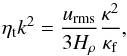 (22)and the growth
rate of NEMPI in that normalization is
(22)and the growth
rate of NEMPI in that normalization is 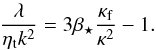 (23)Using β⋆ = 0.23, which is the
relevant value for high magnetic Reynolds numbers (Brandenburg et al. 2012), we find λ/ηtk2 ≈ 2.7−1.3
for κ ≈ 1.1−1.4. However, since Fig. 8 shows an increase of β⋆ with increasing
polytropic index, one might expect a corresponding increase in the growth rate of NEMPI
for a polytropic layer, in which Hρ varies strongly with
height z.
Indeed, in a polytropic atmosphere, Hρ is proportional to
depth. Thus, at any given depth there is a layer beneath, where the stratification is less
strong and the growth rate of NEMPI is lower. In addition, there is a thinner, more
strongly stratified layer above, where NEMPI might grow faster if only the structures
generated by NEMPI have enough room to develop before they touch the top of the atmosphere
at z∞, where the temperature vanishes.
(23)Using β⋆ = 0.23, which is the
relevant value for high magnetic Reynolds numbers (Brandenburg et al. 2012), we find λ/ηtk2 ≈ 2.7−1.3
for κ ≈ 1.1−1.4. However, since Fig. 8 shows an increase of β⋆ with increasing
polytropic index, one might expect a corresponding increase in the growth rate of NEMPI
for a polytropic layer, in which Hρ varies strongly with
height z.
Indeed, in a polytropic atmosphere, Hρ is proportional to
depth. Thus, at any given depth there is a layer beneath, where the stratification is less
strong and the growth rate of NEMPI is lower. In addition, there is a thinner, more
strongly stratified layer above, where NEMPI might grow faster if only the structures
generated by NEMPI have enough room to develop before they touch the top of the atmosphere
at z∞, where the temperature vanishes.
4.2. Mean-field equations
In the following, we consider MFS and compare it with DNS. We also compare our MFS results with those of DNS (Brandenburg et al. 2011; Kemel et al. 2013) using a similar polytropic setup.
The governing equations for the mean quantities (denoted by an overbar) are fairly similar to those for the original equations, except that in the MFS viscosity and magnetic diffusivity are replaced by their turbulent counterparts, and the mean Lorentz force is supplemented by a parameterization of the turbulent contribution to the effective magnetic pressure.
The evolution equations for mean vector potential  , mean
velocity
, mean
velocity  , and
mean density
, and
mean density  , are
, are
![Mathematical equation: \begin{eqnarray} \label{dAmean} &&{\partial\meanAA\over\partial t}=\meanUU\times\meanBB -\etaT\mu_0\meanJJ,\\ \label{dUmean} &&{\meanDD\,\meanUU\over\meanDD t} ={1\over\meanrho}\left[ \meanJJ\times\meanBB+\nab(q_{\rm p}\meanBB^2/2\mu_0)\right] -\nuT\meanQQ-\nab\meanH,\\ &&{\meanDD\,\meanrho\over\meanDD t}=-\meanrho\nab\cdot\meanUU, \end{eqnarray}](/articles/aa/full_html/2014/04/aa22315-13/aa22315-13-eq189.png) Awhere
Awhere
 is the
advective derivative with respect to the mean flow,
the mean
density,
is the
advective derivative with respect to the mean flow,
the mean
density,  the
mean reduced enthalpy,
the
mean reduced enthalpy,  the mean
enthalpy,
the mean
enthalpy,  the mean temperature, Φ the
gravitational potential, ηT = ηt + η,
and νT = νt + ν
are the sums of turbulent and microphysical values of magnetic diffusivity and kinematic
viscosities, respectively. Also,
the mean temperature, Φ the
gravitational potential, ηT = ηt + η,
and νT = νt + ν
are the sums of turbulent and microphysical values of magnetic diffusivity and kinematic
viscosities, respectively. Also,  is the mean current
density, μ0 is the vacuum permeability,
is the mean current
density, μ0 is the vacuum permeability,
 (27)is
a term appearing in the mean viscous force
(27)is
a term appearing in the mean viscous force  ,
where
,
where  is
the traceless rate-of-strain tensor of the mean flow with components
is
the traceless rate-of-strain tensor of the mean flow with components
 ,
and finally the term
,
and finally the term  on the righthand side of Eq.
(25) determines the turbulent
contribution to the effective magnetic pressure. Here, qp depends on
the local field strength; see Eq. (19).
This term enters with a plus sign, so positive values of qp correspond to
a suppression of the total turbulent pressure. The net effect of the mean magnetic field
leads to an effective mean magnetic pressure that becomes negative for qp > 1. This can
indeed be the case for magnetic Reynolds numbers well above unity (Brandenburg et al. 2012); see also Fig. 7 for a polytropic atmosphere.
on the righthand side of Eq.
(25) determines the turbulent
contribution to the effective magnetic pressure. Here, qp depends on
the local field strength; see Eq. (19).
This term enters with a plus sign, so positive values of qp correspond to
a suppression of the total turbulent pressure. The net effect of the mean magnetic field
leads to an effective mean magnetic pressure that becomes negative for qp > 1. This can
indeed be the case for magnetic Reynolds numbers well above unity (Brandenburg et al. 2012); see also Fig. 7 for a polytropic atmosphere.
The boundary conditions for MFS are the same as for DNS, i.e., stress-free for the mean velocity at the top and bottom. For the mean magnetic field, we use either perfect conductor boundary conditions (for horizontal, imposed magnetic fields) or vertical field conditions (for vertical, imposed fields) at the top and bottom. All mean-field variables are assumed to be periodic in the x and y directions. The MFS are performed again with the Pencil Code, which is equipped with a mean-field module for solving the corresponding equations.
4.3. Expected vertical dependence of NEMPI
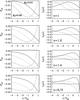 |
Fig. 9 Comparison of |
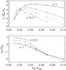 |
Fig. 10 Dependence of growth rate and height where the eigenfunction attains its maximum value (the optimal depth of NEMPI) on field strength from MFS for different values of γ in the presence of a horizontal field for Model I. |
To get an idea about the vertical dependence of NEMPI, we now consider the resulting
dependencies of  ;
see the lefthand panels of Fig. 9. We note that
;
see the lefthand panels of Fig. 9. We note that
 is just a function of β (Eqs. (18) and (19)), which allows us
to approximate the local growth rates as (Rogachevskii
& Kleeorin 2007; Kemel et al.
2013)
is just a function of β (Eqs. (18) and (19)), which allows us
to approximate the local growth rates as (Rogachevskii
& Kleeorin 2007; Kemel et al.
2013)  (28)which are plotted
in the righthand panels of Fig. 9 for Model I.
(28)which are plotted
in the righthand panels of Fig. 9 for Model I.
4.4. Horizontal fields
To analyze the kinematic stage of MFS, we measure the value of the maximum downflow
speed,  at each
height. We then determine the time interval during which the maximum downflow speed
increases exponentially and when the height of the peak is constant and equal to
zB. This yields the
growth rate of the instability as
at each
height. We then determine the time interval during which the maximum downflow speed
increases exponentially and when the height of the peak is constant and equal to
zB. This yields the
growth rate of the instability as  .
.
In Figs. 10 and 11 we plot, respectively for Models I and II, λ (in units of
 ) and
zB versus horizontal
imposed magnetic field strength, B0/Beq.
The maximum growth rates for γ = 5/3 and γ = 1 are similar for both
models (4–5 for Model I and
16–20 for Model II).
It turns out that for γ = 5/3, the growth rate
λ attains a
maximum at some value B0 = Bmax,
and then it decreases with increasing B0, while in an isothermal run
λ is nearly
constant for greater field strength, except near the surface where the proximity to the
boundary is too small. This close proximity reduces the growth rate. For Model I with
γ = 1, the
decline of λ
(toward weaker fields on the lefthand side of the plot) begins when the distance to the
top boundary (ztop − zB ≈ 1.2 Hρ0
for β0 = 0.02) is less than the radius of
magnetic structures (R ≈ 2π/k⊥ ≈ 1.5 Hρ0
using k⊥Hρ0 = 1).
In Model II with γ = 1, the decline of λ occurs for stronger
fields, but the distance to the top boundary (≈1.0 Hρ0) is still
nearly the same as for Model I.
) and
zB versus horizontal
imposed magnetic field strength, B0/Beq.
The maximum growth rates for γ = 5/3 and γ = 1 are similar for both
models (4–5 for Model I and
16–20 for Model II).
It turns out that for γ = 5/3, the growth rate
λ attains a
maximum at some value B0 = Bmax,
and then it decreases with increasing B0, while in an isothermal run
λ is nearly
constant for greater field strength, except near the surface where the proximity to the
boundary is too small. This close proximity reduces the growth rate. For Model I with
γ = 1, the
decline of λ
(toward weaker fields on the lefthand side of the plot) begins when the distance to the
top boundary (ztop − zB ≈ 1.2 Hρ0
for β0 = 0.02) is less than the radius of
magnetic structures (R ≈ 2π/k⊥ ≈ 1.5 Hρ0
using k⊥Hρ0 = 1).
In Model II with γ = 1, the decline of λ occurs for stronger
fields, but the distance to the top boundary (≈1.0 Hρ0) is still
nearly the same as for Model I.
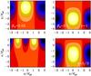 |
Fig. 12 Snapshots of |
In an isothermal layer, the height where the eigenfunction peaks is known to decrease with increasing field strength; see Fig. 6 of Kemel et al. (2012a). One might have expected this decrease to be less steep in the polytropic case, because the optimal depth where NEMPI occurs cannot easily be decreased without suffering a dramatic decrease of the growth rate. This is however not the case, and we find that the optimal depth of NEMPI is now falling off more quickly in Model I, but is more similar for Model II; see the second panels of Figs. 10 and 11. This means that in a polytropic layer, NEMPI works more effectively, and its growth rate is fastest when the magnetic field is not too strong. At the same time, the optimal depth of NEMPI increases, i.e., the resulting value of zB increases as B0 decreases.
The resulting growth rates are somewhat less for Model I and somewhat higher for Model II
than those of earlier mean-field calculations of Kemel et
al. (2012a, their Fig. 6), who found
 in a
model with β⋆ = 0.32 and
βp = 0.05. These differences in the growth
rates are plausibly explained by differences in the mean-field parameters.
in a
model with β⋆ = 0.32 and
βp = 0.05. These differences in the growth
rates are plausibly explained by differences in the mean-field parameters.
Visualizations of the resulting horizontal field structures are shown in Fig. 12 for two values of γ and B0. Increase in the parameter γ results in a stronger localization of the instability at the surface layer, where the density scale height is minimum and the growth of NEMPI is strongest.
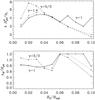 |
Fig. 13 Dependence of growth rate and optimal depth of NEMPI on field strength from MFS for different values of γ in the presence of a vertical field for Model I. |
4.5. Vertical fields
In the presence of a vertical field, the early evolution of the instability is similar to that for a horizontal field. In both cases, the maximum field strength occurs at a somewhat larger depth when saturation is reached, except that shortly before saturation there is a brief interval during which the location of maximum field strength rises slightly upwards in the vertical field case. In the saturated case, however, the flux concentrations from NEMPI are much stronger compared to the case of a horizontal field and it leads to the formation of magnetic flux concentrations of equipartition field strength (Brandenburg et al. 2013, 2014). This is possible because the resulting vertical flux tube is not advected downward with the flow that develops as a consequence of NEMPI. The latter effect is the aforementioned “potato-sack” effect, which acts as a nonlinear saturation mechanism of NEMPI with a horizontal field.
In Figs. 13 and 14 we plot the growth rates λ and the heights where the eigenfunction attains
its maximum values for different β0 = B0/Beq0
for Models I and II, respectively. For γ = 5/3, the maximum growth rate
is higher larger than for γ = 1. This is true for Models I and II, where they
are 8–10 for
γ = 5/3 and
5–7 for
γ = 1. The
nonmonotonous behavior seen in the dependence of λ on B0 is suggestive
of the presence of different mode structures, although a direct inspection of the
resulting magnetic field did not show any obvious differences. However, this irregular
behavior may be related to artifacts resulting from a finite domain size and were not
regarded important enough to justify further investigation.
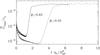 |
Fig. 15 Comparison of |
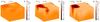 |
Fig. 16 Snapshots from MFS showing |
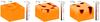 |
Fig. 17 Similar to Fig. 16 of MFS, but for Model II at times similar to those in the DNS of Fig. 5. There are now more structures than in the earlier MFS of Fig. 16, and they develop more rapidly. |
Next we focus on a comparison of the growth rates obtained from MFS for horizontal and vertical fields. The values of β0, zB, and β(zB) = B0/Beq(zB) for horizontal and vertical fields are compared in Table 1 for both models. We see that NEMPI is most effective in regions where the mean magnetic field is a small fraction of the local equipartition field and typically slightly less for γ = 5/3 than for γ = 1. Indeed, for Model I, β(zB) is 3–4% for horizontal fields and 3–6% for vertical fields, while for Model II, β(zB) is 12–17% for horizontal fields and 8–22% for vertical fields. Here, we have used β(zB) = β0e2 − γ(zB/2Hρ0), where eq(x) is the q-exponential function defined by Eq. (3).
Comparison of the optimal depth zB and the corresponding normalized magnetic field strength β(zB) for three values of γ for imposed horizontal and vertical magnetic fields of normalized strengths β0 = B0/Beq0, for Model I.
We expect that higher values of β⋆ will lead to greater
growth rates. To verify this, we compare in Fig. 15
the time evolutions of  for Models I
(with β⋆ = 0.33) and Model II
(with β⋆ = 0.63). The growth
rate has now increased by a factor of 2.4 (from
for Models I
(with β⋆ = 0.33) and Model II
(with β⋆ = 0.63). The growth
rate has now increased by a factor of 2.4 (from  to
9.5), which is slightly more than what is expected from β⋆, which has increased
by a factor of 1.9. This change in the growth rate can also be seen in Fig. 11 and Fig. 14 for
Model II (in comparison with Figs. 10 and 13 for Model I). The dependence of the growth rate on
the magnetic field strength is qualitatively similar for Models I and II. In particular,
it becomes constant for γ = 1, but declines for γ = 5/3
as the field increases. The increase of zB with B0 is, however,
less strong for Model II.
to
9.5), which is slightly more than what is expected from β⋆, which has increased
by a factor of 1.9. This change in the growth rate can also be seen in Fig. 11 and Fig. 14 for
Model II (in comparison with Figs. 10 and 13 for Model I). The dependence of the growth rate on
the magnetic field strength is qualitatively similar for Models I and II. In particular,
it becomes constant for γ = 1, but declines for γ = 5/3
as the field increases. The increase of zB with B0 is, however,
less strong for Model II.
Snapshots of from MFS for
γ = 5/3 and β0 = 0.05 at
different times for Model I are shown in Fig. 16.
Comparison with the results of MFS for Model II (see Fig. 17) shows that Model II fits the DNS better. This is also seen by comparing Fig.
17 with Fig. 5. However, our basic conclusions formulated in this paper are not affected.
5. Conclusions
The present work has demonstrated that in a polytropic layer, both in MFS and DNS, NEMPI develops primarily in the uppermost layers, provided the mean magnetic field is not too strong. If the field gets stronger, NEMPI can still develop, but the magnetic structures now occur at greater depths and the growth rate of NEMPI is lower. However, at some point when the magnetic field gets too strong, NEMPI is suppressed in the case of a polytropic layer, while it would still operate in the isothermal case, provided the domain is deep enough. The slow down of NEMPI is not directly a consequence of a longer turnover time at greater depths, but it is related to stratification being too weak for NEMPI to be excited.
By and large, the scaling relations determined previously for isothermal layers with constant scale height still seem to apply locally to polytropic layers with variable scale heights. In particular, the horizontal scale of structures was previously determined to be about 6–8 Hρ (Kemel et al. 2013; Brandenburg et al. 2014). Looking now at Fig. 4, we see that for β0 = 0.02 and γ = 5/3, the structures have a wavelength of ≈3 Hρ0, but this is at a depth where Hρ ≈ 0.3 Hρ0. Thus, locally we have a wavelength of ≈10 Hρ. The situation is similar in the next panel of Fig. 4 where the wavelength is ≈6 Hρ0, and the structures are at a depth where Hρ ≈ 1.5 Hρ0, so locally we have a wavelength of ≈9 Hρ. We can therefore conclude that our earlier results for isothermal layers can still be applied locally to polytropic layers.
A new aspect, however, that was not yet anticipated at the time, concerns the importance of NEMPI for vertical fields. While NEMPI with horizontal magnetic field still leads to downflows in the nonlinear regime (the “potato-sack” effect), our present work now confirms that structures consisting of vertical fields do not sink, but reach a strength comparable to or in excess of the equipartition value (Brandenburg et al. 2013, 2014). This makes NEMPI a viable mechanism for spontaneously producing magnetic spots in the surface layers. Our present study therefore supports ideas about a shallow origin for active regions and sunspots (Brandenburg 2005; Brandenburg et al. 2010; Kitiashvili et al. 2010; Stein & Nordlund 2012), contrary to common thinking that sunspots form near the bottom of the convective zone (Parker 1975; Spiegel & Weiss 1980; D’Silva & Choudhuri 1993). More specifically, the studies of Losada et al. (2013) point toward the possibility that magnetic flux concentrations form in the top 6 Mm, i.e., in the upper part of the supergranulation layer.
There are obviously many other issues of NEMPI that need to be understood before it can be
applied in a meaningful way to the formation of active regions and sunspots. One question is
whether the hydrogen ionization layer and the resulting H− opacity in the upper layers of
the Sun are important in providing a sharp temperature drop and whether this would enhance
the growth rate of NEMPI, just like strong density stratification does. Another important
question concerns the relevance of a radiating surface, which also enhances the density
contrast. Finally, of course, one needs to verify that the assumption of forced turbulence
is useful in representing stellar convection. Many groups have considered magnetic flux
concentrations using realistic turbulent convection (Kitiashvili et al. 2010; Rempel 2011; Stein & Nordlund 2012). However, only at
sufficiently large resolution can one expect strong enough scale separation between the
scale of the smallest eddies and the size of magnetic structures. That is why forced
turbulence has an advantage over convection. Ultimately, however, such assumptions should no
longer be necessary. On the other hand, if scale separation is poor, our present
parameterization might no longer be accurate enough, and one would need to replace the
multiplication between qp and
 in Eq. (25) by a convolution. This possibility is fairly
speculative and requires a separate investigation. Nevertheless, in spite of these issues,
it is important to emphasize that the qualitative agreement between DNS and MFS is already
surprisingly good.
in Eq. (25) by a convolution. This possibility is fairly
speculative and requires a separate investigation. Nevertheless, in spite of these issues,
it is important to emphasize that the qualitative agreement between DNS and MFS is already
surprisingly good.
Acknowledgments
This work was supported in part by the European Research Council under the AstroDyn Research Project No. 227952, by the Swedish Research Council under the project grants 621-2011-5076 and 2012-5797 (I.R.L., A.B.), by EU COST Action MP0806, by the European Research Council under the Atmospheric Research Project No. 227915, and by a grant from the Government of the Russian Federation under contract No. 11.G34.31.0048 (N.K., I.R.). We acknowledge the allocation of computing resources provided by the Swedish National Allocations Committee at the Center for Parallel Computers at the Royal Institute of Technology in Stockholm and the National Supercomputer Centers in Linköping, the High Performance Computing Center North in Umeå, and the Nordic High Performance Computing Center in Reykjavik.
References
- Brandenburg, A. 2005, ApJ, 625, 539 [Google Scholar]
- Brandenburg, A., Kleeorin, N., & Rogachevskii, I. 2010, Astron. Nachr., 331, 5 [NASA ADS] [CrossRef] [Google Scholar]
- Brandenburg, A., Kemel, K., Kleeorin, N., Mitra, D., & Rogachevskii, I. 2011, ApJ, 740, L50 [NASA ADS] [CrossRef] [Google Scholar]
- Brandenburg, A., Kemel, K., Kleeorin, N., & Rogachevskii, I. 2012, ApJ, 749, 179 [NASA ADS] [CrossRef] [Google Scholar]
- Brandenburg, A., Kleeorin, N., & Rogachevskii, I. 2013, ApJ, 776, L23 [NASA ADS] [CrossRef] [Google Scholar]
- Brandenburg, A., Gressel, O., Jabbari, S., Kleeorin, N., & Rogachevskii, I. 2014, A&A, 562, A53 [NASA ADS] [CrossRef] [EDP Sciences] [Google Scholar]
- D’Silva, S., & Choudhuri, A. R. 1993, A&A, 272, 621 [NASA ADS] [Google Scholar]
- Jabbari, S., Brandenburg, A., Kleeorin, N., Mitra, D., & Rogachevskii, I. 2013, A&A, 556, A106 [NASA ADS] [CrossRef] [EDP Sciences] [Google Scholar]
- Käpylä, P. J., Brandenburg, A., Kleeorin, N., Mantere, M. J., & Rogachevskii, I. 2012, MNRAS, 422, 2465 [NASA ADS] [CrossRef] [Google Scholar]
- Kemel, K., Brandenburg, A., Kleeorin, N., & Rogachevskii, I. 2012a, Astron. Nachr., 333, 95 [NASA ADS] [CrossRef] [Google Scholar]
- Kemel, K., Brandenburg, A., Kleeorin, N., Mitra, D., & Rogachevskii, I. 2012b, Sol. Phys., 280, 321 [NASA ADS] [CrossRef] [Google Scholar]
- Kemel, K., Brandenburg, A., Kleeorin, N., Mitra, D., & Rogachevskii, I. 2013, Sol. Phys., 287, 293 [NASA ADS] [CrossRef] [Google Scholar]
- Kitiashvili, I. N., Kosovichev, A. G., Wray, A. A., & Mansour, N. N. 2010, ApJ, 719, 307 [NASA ADS] [CrossRef] [Google Scholar]
- Kleeorin, N., & Rogachevskii, I. 1994, Phys. Rev. E, 50, 2716 [NASA ADS] [CrossRef] [Google Scholar]
- Kleeorin, N. I., Rogachevskii, I. V., & Ruzmaikin, A. A. 1989, Sov. Astron. Lett., 15, 274 [NASA ADS] [Google Scholar]
- Kleeorin, N. I., Rogachevskii, I. V., & Ruzmaikin, A. A. 1990, Sov. Phys. JETP, 70, 878 [Google Scholar]
- Kleeorin, N., Mond, M., & Rogachevskii, I. 1993, Phys. Fluids B, 5, 4128 [NASA ADS] [CrossRef] [Google Scholar]
- Kleeorin, N., Mond, M., & Rogachevskii, I. 1996, A&A, 307, 293 [NASA ADS] [Google Scholar]
- Krause, F., & Rädler, K.-H. 1980, Mean-field Magnetohydrodynamics and Dynamo Theory (Oxford: Pergamon Press) [Google Scholar]
- Losada, I. R., Brandenburg, A., Kleeorin, N., Mitra, D., & Rogachevskii, I. 2012, A&A, 548, A49 [NASA ADS] [CrossRef] [EDP Sciences] [Google Scholar]
- Losada, I. R., Brandenburg, A., Kleeorin, N., & Rogachevskii, I. 2013, A&A, 556, A83 [NASA ADS] [CrossRef] [EDP Sciences] [Google Scholar]
- Newcomb, W. A. 1961, Phys. Fluids, 4, 391 [NASA ADS] [CrossRef] [MathSciNet] [Google Scholar]
- Parker, E. N. 1955, ApJ, 121, 491 [NASA ADS] [CrossRef] [Google Scholar]
- Parker, E. N. 1966, ApJ, 145, 811 [NASA ADS] [CrossRef] [Google Scholar]
- Parker, E. N. 1975, ApJ, 198, 205 [NASA ADS] [CrossRef] [Google Scholar]
- Plastino, A. R., & Plastino, A. 1993, Phys. Lett. A, 174, 384 [NASA ADS] [CrossRef] [MathSciNet] [Google Scholar]
- Rempel, M. 2011, ApJ, 740, 15 [NASA ADS] [CrossRef] [Google Scholar]
- Rogachevskii, I., & Kleeorin, N. 2007, Phys. Rev. E, 76, 056307 [NASA ADS] [CrossRef] [Google Scholar]
- Spiegel, E. A., & Weiss, N. O. 1980, Nature, 287, 616 [CrossRef] [Google Scholar]
- Spruit, H. C. 1981, A&A, 98, 155 [NASA ADS] [Google Scholar]
- Schüssler, M., Caligari, P., Ferriz-Mas, A., & Moreno-Insertis, F. 1994, A&A, 281, L69 [Google Scholar]
- Stein, R. F., & Nordlund, Å. 2012, ApJ, 753, L13 [Google Scholar]
- Sur, S., Brandenburg, A., & Subramanian, K. 2008, MNRAS, 385, L15 [NASA ADS] [CrossRef] [Google Scholar]
- Tsallis, C. 1988, J. Stat. Phys., 52, 479 [NASA ADS] [CrossRef] [MathSciNet] [Google Scholar]
- Vitense, E. 1953, Z. Astrophys., 32, 135 [NASA ADS] [Google Scholar]
- Yamano, T. 2002, Stat. Mech. Appl., 305, 486 [CrossRef] [Google Scholar]
- Warnecke, J., Losada, I. R., Brandenburg, A., Kleeorin, N., & Rogachevskii, I. 2013, ApJ, 777, L37 [NASA ADS] [CrossRef] [Google Scholar]
All Tables
Comparison of the optimal depth zB and the corresponding normalized magnetic field strength β(zB) for three values of γ for imposed horizontal and vertical magnetic fields of normalized strengths β0 = B0/Beq0, for Model I.
All Figures
|
Fig. 1 Isothermal and polytropic relations for different values of γ when calculated using the conventional formula ρ ∝ (z∞ − z)n with n = 1/(γ − 1). |
| In the text | |
|
Fig. 2 Polytropes (Eq. (4)) with γ = 1 (solid line), 1.2 (dash-dotted), 1.4 (dotted), and 5/3 (dashed) and density scale height (Eq. (5)) for −4 ≤ −z/Hρ0 ≤ 1.2. The total density contrast is similar for γ = 1 and 5/3. |
| In the text | |
|
Fig. 3 Sketch showing the expected size distribution of the nearly circular NEMPI eigenfunction structures at different heights. |
| In the text | |
|
Fig. 4 Snapshots of |
| In the text | |
|
Fig. 5 Snapshots from DNS showing |
| In the text | |
|
Fig. 6 Cuts of Bz/Beq(z) in (a) the xy plane at the top boundary (z/Hρ0 = 1.2) and (b) the xz plane through the middle of the spot at y = 0 for γ = 5/3 and β0 = 0.05. In the xz cut, we also show magnetic field lines and flow vectors obtained by numerically averaging in azimuth around the spot axis. |
| In the text | |
|
Fig. 7 Effective magnetic pressure obtained from DNS in a polytropic layer with different γ for horizontal (H, red curves) and vertical (V, blue curves) mean magnetic fields. |
| In the text | |
|
Fig. 8 Parameters qp0, βp, and β⋆ for the function qp(β) (see Eq. (19)) versus γ for horizontal (red line) and vertical (blue line) mean magnetic fields. |
| In the text | |
|
Fig. 9 Comparison of |
| In the text | |
|
Fig. 10 Dependence of growth rate and height where the eigenfunction attains its maximum value (the optimal depth of NEMPI) on field strength from MFS for different values of γ in the presence of a horizontal field for Model I. |
| In the text | |
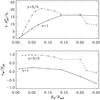 |
Fig. 11 Same as Fig. 10 (horizontal field), but for Model II. |
| In the text | |
|
Fig. 12 Snapshots of |
| In the text | |
|
Fig. 13 Dependence of growth rate and optimal depth of NEMPI on field strength from MFS for different values of γ in the presence of a vertical field for Model I. |
| In the text | |
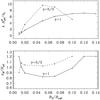 |
Fig. 14 Same as Fig. 13 (vertical field), but for Model II. |
| In the text | |
|
Fig. 15 Comparison of |
| In the text | |
|
Fig. 16 Snapshots from MFS showing |
| In the text | |
|
Fig. 17 Similar to Fig. 16 of MFS, but for Model II at times similar to those in the DNS of Fig. 5. There are now more structures than in the earlier MFS of Fig. 16, and they develop more rapidly. |
| In the text | |
Current usage metrics show cumulative count of Article Views (full-text article views including HTML views, PDF and ePub downloads, according to the available data) and Abstracts Views on Vision4Press platform.
Data correspond to usage on the plateform after 2015. The current usage metrics is available 48-96 hours after online publication and is updated daily on week days.
Initial download of the metrics may take a while.