| Issue |
A&A
Volume 563, March 2014
|
|
|---|---|---|
| Article Number | A128 | |
| Number of page(s) | 9 | |
| Section | Galactic structure, stellar clusters and populations | |
| DOI | https://doi.org/10.1051/0004-6361/201423505 | |
| Published online | 21 March 2014 | |
Milky Way rotation curve from proper motions of red clump giants
1
Instituto de Astrofísica de Canarias,
38200
La Laguna, Tenerife
Spain
e-mail:
This email address is being protected from spambots. You need JavaScript enabled to view it.
2
Departamento de Astrofísica, Universidad de La
Laguna, 38206, La
Laguna, Tenerife,
Spain
Received:
24
January
2014
Accepted:
9
February
2014
Abstract
Aims. We derive the stellar rotation curve of the Galaxy in the range of Galactocentric radii of R = 4−16 kpc at different vertical heights from the Galactic plane of z between –2 and +2 kpc. With this we reach high Galactocentric distances in which the kinematics is poorly known due mainly to uncertainties in the distances to the sources.
Methods. We used the PPMXL survey, which contains the USNO-B1 proper motions catalog cross–correlated with the astrometry and near-infrared photometry of the 2MASS Point Source Catalog. To improve the accuracy of the proper motions, we calculated the average proper motions of quasars to know their systematic shift from zero in this PPMXL survey, and we applied the corresponding correction to the proper motions of the whole survey, which reduces the systematic error. We selected from the color–magnitude diagram K vs. (J − K) the standard candles corresponding to red clump giants and used the information of their proper motions to build a map of the rotation speed of our Galaxy.
Results. We obtain an almost flat rotation curve with a slight decrease for higher values of R or |z|. The most puzzling result is obtained for the farthest removed and most off-plane regions, that is, at R ≈ 16 kpc and |z| ≈ 2 kpc, where a significant deviation from a null average proper motion (~4 mas/yr) in the Galactic longitude direction for the anticenter regions can be directly translated into a rotation speed much lower than at the solar Galactocentric radius. In particular, we obtain an average speed of 82 ± 5(stat.) ± 58(syst.) km s-1 (assuming a solar Galactocentric distance of 8 kpc, and a circular/azimuthal velocity of 250 km s-1 for the Sun and of 238 km s-1 for the Local Standard of Rest), where the high systematic error bar is due mainly to the highest possible contamination of non-red clump giants and the proper motion systematic uncertainty.
Conclusions. A scenario with a rotation speed lower than 150 km s-1 in these farthest removed and most off-plane regions of our explored zone is intriguing, and invites one to reconsider different possibilities for the dark matter distribution. However, given the high systematic errors, we cannot conclude about this. Hence, more measurements of the proper motions at high R and |z| are necessary to validate the exotic scenario that would arise if this low speed were confirmed.
Key words: Galaxy: kinematics and dynamics / Galaxy: disk
© ESO, 2014
1. Introduction
The rotation curve of the Milky Way disk was obtained using many different tracers and within different Galactocentric distance ranges. Dias & Lépine (2005) determined the rotation speed of the spiral pattern of the Galaxy by direct observation of the birthplaces of open clusters of stars in the Galactic disk as a function of their age, confirming that the spiral arms rotate like a rigid body, as predicted by the classical theory of spiral waves. Bobylev et al. (2008) used space velocities of young open star clusters and the radial velocities of HI clouds and star-forming regions to derive the Galactic rotation curve in the range of 3 < R(kpc)< 12; a more recent study by Reid et al. (2014) used proper motions of in-plane star-forming regions in radio and reached R ≈ 16 kpc. Bovy et al. (2012) measured a flat rotation curve in the range 4 < R(kpc)< 14 by fitting the radial velocities of some stars. Compilations of other rotation curve measurements are given by Sofue et al. (2009) and Bhattacharjee et al. (2013) and references therein.
In general, the outer rotation curve of the stellar population is more poorly determined mainly because of the inaccuracy in the distance determination to the stars or other sources (Sofue 2011), and we wish to improve this here. We use the red clump giant (RCG) population, which is a very appropriate standard candle (e.g., Castellani et al. 1992) with relatively low error bars on its distance estimate, and can be observed up to distances of ≈8 kpc, which allows one to reach R ≲ 16 kpc (López-Corredoira et al. 2002). Williams et al. (2013) have used RCGs to derive this kinematical information, but only within the range 6 < R(kpc)< 10, |z| < 2 kpc, which does not reach the farthest regions of the stellar disk we aim to explore here. To derive the Milky Way rotation curve from proper motions of RCGs in the range 4 < R(kpc)< 16 for |z| < 2 kpc.
The tool we used for our analysis of kinematics is a catalog of proper motions. Bond et al. (2010) have also made an extended analysis of the stellar kinematics, including the rotation speed, from proper motions with a revised version of the catalog SDSS-DR7. Aihara et al. (2011) reported later that there were significant problems with the measurement of the astrometry of SDSS-DR8 and previous versions, which in turn leads to problems with their proper motions as well, but Bond et al. (2010) may have taken them into account by analyzing the proper motion of quasars. Nonetheless, this analysis of the SDSS-DR7 survey does not cover the Galactic plane at | b| < 20°, therefore it cannot be used to explore high values of R. Reid et al. (2014), as said, also analyze proper motions, but only for in-plane regions. Here we concentrate on the region | b| < 20°.
The structure of this paper is as follows: in Sect. 2 the data source is described; the method to subtract the RCG stars is detailed in Sect. 3; the rotation curve from proper motions is calculated in Sect. 4, with an extra section on how to correct for the systematic errors of proper motions in Sect. 5; this leads to the results in Sect. 6 and their dynamical consequences in Sect. 7. A summary and conclusions are presented in the last section. Unless specified otherwise we assumed for the Sun a Galactocentric distance of 8 kpc and a circular/azimuthal velocity of 250 km s-1, and a circular/azimuthal velocity of the Local Standard of Rest (LSR) of 238 km s-1.
2. Data from the star catalog PPMXL: subsample of 2MASS
The star catalog PPMXL (Roeser et al. 2010) lists positions and proper motions of about 900 million objects, aiming to be complete for the whole sky down to magnitude V ≈ 20. It is the result of the re-reduction of the catalog of astrometry, visible photometry and proper motions of the USNO-B1 catalog cross–correlated with the astrometry and near infrared photometry of the 2MASS Point-Source Catalog, and re-calculating the proper motions in the absolute reference frame of International Celestial Reference Frame (ICRS), with respect to the barycenter of the solar system. The typical statistical errors of these proper motion is 4–10 mas/yr while the systematic errors are on average 1–2 mas/yr. From the whole PPMXL, we first selected the subsample of 2MASS sources with mK ≤ 14 and available J photometry. This yielded a total of 126 636 484 objects with proper motions, i.e. an average of 3100 sources deg-2.
3. Selection of red clump giants
From these data, we selected the red clump giants (RCGs) in K vs. J − K color–magnitude diagrams. Near-infrared color magnitude diagrams are very suitable for separating the RCGs because of their clear separation of the dwarf population up to magnitude mK ≲ 13 (López-Corredoira et al. 2002). Moreover, the absolute magnitudes vary only little in the near-infrared with metallicity or age (Castellani et al. 1992; Pietrzyński et al. 2003). This narrow luminosity function distribution (Castellani et al. 1992) makes them very appropriate standard candles that trace the old stellar population of the Galactic structure.
Here we used the same selection method for RCGs as in López-Corredoira et al. (2002). For each magnitude mK,0 we determined the
(J − K)0 which gives the
highest count density along this horizontal line of the color–magnitude diagram for the RCG,
and we considered all the stars within the rectangle with points [(J − K),mK]
such that ![Mathematical equation: \begin{eqnarray} &&m_{K,0}-\Delta m_K \le m_K \le m_{K,0}+\Delta m_K,\nonumber\\ &&{\rm Max}[(J-K)_{{\rm red\ clump}}(J-K)_0-\Delta (J-K)]\le (J-K) \\ &&\le (J-K)_0+\Delta (J-K). \end{eqnarray}](/articles/aa/full_html/2014/03/aa23505-14/aa23505-14-eq34.png) We
take ΔmK = Δ(J − K) =0.2
mag. Examples are given in Fig. 1 and in the top panel
of 8. Here, we ran the same application for the whole
area of the sky with | b| ≤ 20° in bins of Δℓ = 1°,
Δb = 1° and 9.8 < mK,0 ≤ 13.0
in bins with ΔmK,0 = 0.4 mag. We did
not investigate fields with b > 20° because we
are interested in the disk stars at low z; we did not not analyze either the brighter stars
with mK,0 < 9.8,
because there are very few to accumulate statistics, nor the fainter stars with
mK,0 > 13.0
because they have higher ratio of dwarf contamination. We selected only bins with more than
ten sources. In total the number of RCGs with these criteria is 19 189 177 in an area of
14 100 square degrees, that is, an average of 1360 RCGs per square degree.
We
take ΔmK = Δ(J − K) =0.2
mag. Examples are given in Fig. 1 and in the top panel
of 8. Here, we ran the same application for the whole
area of the sky with | b| ≤ 20° in bins of Δℓ = 1°,
Δb = 1° and 9.8 < mK,0 ≤ 13.0
in bins with ΔmK,0 = 0.4 mag. We did
not investigate fields with b > 20° because we
are interested in the disk stars at low z; we did not not analyze either the brighter stars
with mK,0 < 9.8,
because there are very few to accumulate statistics, nor the fainter stars with
mK,0 > 13.0
because they have higher ratio of dwarf contamination. We selected only bins with more than
ten sources. In total the number of RCGs with these criteria is 19 189 177 in an area of
14 100 square degrees, that is, an average of 1360 RCGs per square degree.
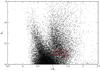 |
Fig. 1 Example of application of RCG selection from PPMXL survey in a K vs. J − K color–magnitude diagram. This case is for the direction ℓ = 125°, b = 2°, at one particular K-magnitude mK,0 = 13.0, giving a maximum of counts within RCG region at (J − K)0 = 1.25. The dashed rectangle represents the area where the RCGs are selected. |
Then, for each bin of RCGs with a given (ℓ, b, mK,0, (J − K)0) we can derive its
cumulative extinction along the line of sight and its 3D position in the Galaxy
(x,
y,
z). The
extinction and distance follow (López-Corredoira et al. 2002, Sect. 3): ![Mathematical equation: \begin{eqnarray} A_K&=&0.67[(J\!-\!K)_0\!-\!(J-K)_{{\rm red\ clump}}]\, \text{(Marshall et~al. 2006)},\quad\quad\\ r&=&10^{\frac{m_{K,0}-M_{K,{\rm red\ clump}}+5-A_K}{5}}\cdot \end{eqnarray}](/articles/aa/full_html/2014/03/aa23505-14/aa23505-14-eq52.png) We
used the updated parameter values: MK,red clump = −1.60,
(J − K)red clump = 0.62
(averages of the values given by Laney et al. 2012
and Yaz Gökçe et al. 2013) and Galactocentric
distance of the Sun R⊙ = 8 kpc (Malkin 2013); we neglected the height of the Sun over the plane. We did not
consider any error in the distance determination because of the error in the absolute
magnitude of the RCGs, which is expected to be negligible in the outer disk: in the worst of
the cases with mK = 13.0, typical
uncertainties of ≲0.02 mag in
the RCG absolute magnitude (Laney et al. 2012; Yaz
Gökçe et al. 2013), plus the determination inaccuracy
of the average absolute magnitude on the order of 0.007 (for a typical number of stars per
bin of 400, and Δm = 0.2), it leads to relative errors in the distance
of 1% for distances of around 8 kpc, and gives a negligible error of ~5 km s-1 in the determination of the
rotation curve (Sofue 2011, Fig. 5 multiplied by one
half). For lower magnitudes the number of stars per bin is lower, which produces higher
relative errors of the distance, but the error produced in the rotation curve is much lower
(Sofue 2011, Fig. 5). We do not know the extinction
uncertainty; assuming errors of up to 0.02 mag in K in the outer disk, we derive the same
negligible uncertainties, except perhaps in the very few regions strictly in the plane
(z = 0) where
the error might be somewhat larger. In the inner disk, the errors may be larger, both
because of higher extinction and because of higher values of uncertainty of the rotation
speed for a given relative error of distances (Sofue 2011, Fig. 5), but these are smaller than other statistical and systematic errors
we derive.
We
used the updated parameter values: MK,red clump = −1.60,
(J − K)red clump = 0.62
(averages of the values given by Laney et al. 2012
and Yaz Gökçe et al. 2013) and Galactocentric
distance of the Sun R⊙ = 8 kpc (Malkin 2013); we neglected the height of the Sun over the plane. We did not
consider any error in the distance determination because of the error in the absolute
magnitude of the RCGs, which is expected to be negligible in the outer disk: in the worst of
the cases with mK = 13.0, typical
uncertainties of ≲0.02 mag in
the RCG absolute magnitude (Laney et al. 2012; Yaz
Gökçe et al. 2013), plus the determination inaccuracy
of the average absolute magnitude on the order of 0.007 (for a typical number of stars per
bin of 400, and Δm = 0.2), it leads to relative errors in the distance
of 1% for distances of around 8 kpc, and gives a negligible error of ~5 km s-1 in the determination of the
rotation curve (Sofue 2011, Fig. 5 multiplied by one
half). For lower magnitudes the number of stars per bin is lower, which produces higher
relative errors of the distance, but the error produced in the rotation curve is much lower
(Sofue 2011, Fig. 5). We do not know the extinction
uncertainty; assuming errors of up to 0.02 mag in K in the outer disk, we derive the same
negligible uncertainties, except perhaps in the very few regions strictly in the plane
(z = 0) where
the error might be somewhat larger. In the inner disk, the errors may be larger, both
because of higher extinction and because of higher values of uncertainty of the rotation
speed for a given relative error of distances (Sofue 2011, Fig. 5), but these are smaller than other statistical and systematic errors
we derive.
3.1. Contamination
Our selected sources (almost 20 million) are mostly RCGs but there is also a small fraction of contamination. These sources are:
-
Extragalactic sources: they are on average ≈13 galaxies/deg2 up to magnitude mK = 13.2 (14.4 with mK ≤ 13.5, López-Corredoira & Betancort-Rijo 2004; with the correction for a differential galaxy count of about five galaxies/deg2/mag at mK = 13.3, Cole et al. 2001), with fluctuations
 in areas of one square
degree (López-Corredoira & Betancort-Rijo 2004). This is negligible in comparison with the density of stars.
Nonetheless, the contamination is even much lower because within this range of
magnitudes most of them are extended objects, which are not included in Point Source
Catalog of 2MASS. The most important extragalactic contamination stems from quasars,
which are ≲0.05
deg-2 up to
magnitude mK = 13.2 (from
the data by Wu et al. 2011; see Sect. 5), and there are fewer of them with the same
colors as giant stars. This is again negligible compared with the average 1360 RCG
stars per square degree in our fields. Therefore, we consider that this very small
contamination does not affect our results significantly.
in areas of one square
degree (López-Corredoira & Betancort-Rijo 2004). This is negligible in comparison with the density of stars.
Nonetheless, the contamination is even much lower because within this range of
magnitudes most of them are extended objects, which are not included in Point Source
Catalog of 2MASS. The most important extragalactic contamination stems from quasars,
which are ≲0.05
deg-2 up to
magnitude mK = 13.2 (from
the data by Wu et al. 2011; see Sect. 5), and there are fewer of them with the same
colors as giant stars. This is again negligible compared with the average 1360 RCG
stars per square degree in our fields. Therefore, we consider that this very small
contamination does not affect our results significantly. -
Main-sequence stars: there is some contamination of the dwarfs from the main sequence: for the faintest bin of magnitude (mK = 13), ≲10% of the stars in our selected sample of RCGs might indeed be main-sequence dwarfs (López-Corredoira et al. 2002, Sect. 3.3.3); for brighter magnitudes, the contamination is lower. Indeed, the contamination might be slightly lower because we added an extra-constraint: here (J − K) > 0.62, which avoids the contact with the main sequence in regions of low extinction, whereas in López-Corredoira et al. (2002) the minimum of (J − K) was 0.55.
-
Other types of giant stars: there may be some giants that are not RCGs in our selected sample: M giants, asymptotic giant branch bump stars and red giant branch bump (RGBB) stars (Nataf et al. 2013). They are negligible except for the third one (RGBB), which has absolute magnitudes MK between +2.0 and –1.4 (López-Corredoira et al. 2002, Sect. 3.3.2) with a peak around 0.8 mag fainter than the RCG peak (Wegg & Gerhard 2013; they analyzed the RCG for the bulge, but there are no significant differences with the RCG luminosity function in the disk). According to Wegg & Gerhard (2013), the luminosity function at the observed color yields about 20% RGGB stars with respect to the RCG stars at a given distance (this is a 16.7% of the total of RGGB+RCG). Because the distances of both populations are related by rRGGB = 0.7 rRCG (derived from the difference of 0.8 mag) and the number of observed stars at a given distance is proportional to N(r) = N(1)r3ρ(r), where N(r) is a monotonously decreasing function (because the number of RCGs increases with magnitude; see Fig. 1 or in the top panel of 8. Usually,
 is between 0.4 and 0.7) and we derive a contamination of RGBBs of ≲10% as well.
The contamination of the last two items is important for calculating the average proper motions, because dwarfs are much closer than RCGs, and attributing an incorrect distance by a factor f would imply multiplying its real proper motion by a factor f, which in turn would mean huge linear velocities for these dwarfs and a considerably increased average if there is some net average velocity of these dwarfs. But this can be improved by using the median of the proper motions instead of the average of proper motions and by bearing in mind that there might be a systematic error due to this contamination, which would move the median to the position of the ordered set of proper motions in the range of 40–60% instead of 50%. See the discussion in Sect. 7.
3.2. Proper motion of the RCGs
From the mean 3D position of the bin with (ℓ, b, mK,0) with a number
N of RCG
stars, we calculated its median proper motion in Galactic coordinates: μℓ, μb. The angular proper
motion is, of course, directly converted into a linear velocity proper motion
(vℓ, vb) simply by multiplying
μℓcosb
and μb by its distance from
the Sun. Only bins with N > 10 are included in the
calculation. We found the use of the median instead of the average more appropriate
because, as said in the previous subsection, it is a better way to exclude the outliers
because of all kind of errors. The statistical error bars of the median were calculated
for a 95% C.L.: the upper and lower limits correspond to the positions
 of the ordered set of N data. Since the errors of the averages are
evaluated by a χ2 analysis, the confidence level
associated to these error bars is not important at this stage; their inverse square was
just used as weight in the weighted averages of multiple bins and the error bar of these
averages were quantified from the dispersion. Moreover, as said above, we calculated a
systematic error due to contamination: the upper and lower limits correspond to the
positions 0.5N ± 0.1N of the ordered set of
N data
(assuming the worst cases in which the contamination of non-RCGs is 20% and that the
proper motions of these non-RCGs are all higher or lower than the median).
of the ordered set of N data. Since the errors of the averages are
evaluated by a χ2 analysis, the confidence level
associated to these error bars is not important at this stage; their inverse square was
just used as weight in the weighted averages of multiple bins and the error bar of these
averages were quantified from the dispersion. Moreover, as said above, we calculated a
systematic error due to contamination: the upper and lower limits correspond to the
positions 0.5N ± 0.1N of the ordered set of
N data
(assuming the worst cases in which the contamination of non-RCGs is 20% and that the
proper motions of these non-RCGs are all higher or lower than the median).
4. Deriving the rotation curve from proper motions
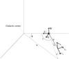 |
Fig. 2 Representation of kinematics of a star with respect to the Sun. |
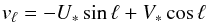
The 3D velocity of the combination of radial velocity (vr) and proper motions
(vℓ, vb) is related to the
velocity in the reference system U, V, W as plotted in Fig. 2 by  (5)
(5)
 where
(U∗,V∗,W∗)
is the velocity of a star relative to the Sun in the system (U,V,W). The Sun velocity in
this system with respect to the Galactic center is (U⊙,Vg, ⊙,W⊙);
the second coordinate
where
(U∗,V∗,W∗)
is the velocity of a star relative to the Sun in the system (U,V,W). The Sun velocity in
this system with respect to the Galactic center is (U⊙,Vg, ⊙,W⊙);
the second coordinate 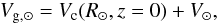 (6)where
Vc(R⊙,z = 0)
is the rotation speed of the Local Standard of Rest with respect to the Galactic center;
(U⊙,V⊙,W⊙)
is the velocity of the Sun with respect to the LSR. Here, we adopted the values
U⊙ = 14.0 ± 1.5 km s-1, V⊙ = 12 ± 2
km s-1 and
W⊙ = 6 ± 2 km s-1 (Schönrich 2012). We used two values of Vg, ⊙: 250 ± 9 km s-1 (Schönrich 2012) and 200 km s-1 (the minimum value in the literature; see McMillan
& Binney 2010; Bhattacharjee et al. 2013).
(6)where
Vc(R⊙,z = 0)
is the rotation speed of the Local Standard of Rest with respect to the Galactic center;
(U⊙,V⊙,W⊙)
is the velocity of the Sun with respect to the LSR. Here, we adopted the values
U⊙ = 14.0 ± 1.5 km s-1, V⊙ = 12 ± 2
km s-1 and
W⊙ = 6 ± 2 km s-1 (Schönrich 2012). We used two values of Vg, ⊙: 250 ± 9 km s-1 (Schönrich 2012) and 200 km s-1 (the minimum value in the literature; see McMillan
& Binney 2010; Bhattacharjee et al. 2013).
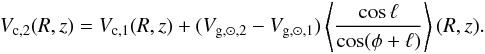
Assuming average circular orbits with rotation speed Vc(R,z) at Galactocentric
radius R,
independent of the azimuth φ, the coplanar velocities of the star with respect to
the Sun are  (7)
(7) where
φ is the
Galactocentric azimuth of the star. We did not consider an asymmetric drift in each orbit
(e.g., Golubov et al. 2013) because of the
differences with perfect circular orbits: we cannot determine with enough precision the
intrinsic velocity dispersion necessary for calculating the asymmetric drift, because the
measurement errors in the proper motions dominate, and, in any case, the expected correction
value is lower than 5% (Bovy et al. 2012, Fig. 4
bottom panel), which is lower than our typical error bars for the rotation speed. We did not
consider the Galactic warp either: if we had considered the warp modeled as a set of
circular rings that are rotated and whose orbit is in a plane with angle iw(R)
with respect to the Galactic plane, then the terms Vc(R,z) in Eq. (7) would need to be multiplied by a factor
cos [iw(R)cos(φ − φw)],
where φw is the azimuth of line
of nodes. The maximum elevation of the stellar warp at R = 16 kpc is z ~ 1 kpc (Reylé et al. 2009), which gives
where
φ is the
Galactocentric azimuth of the star. We did not consider an asymmetric drift in each orbit
(e.g., Golubov et al. 2013) because of the
differences with perfect circular orbits: we cannot determine with enough precision the
intrinsic velocity dispersion necessary for calculating the asymmetric drift, because the
measurement errors in the proper motions dominate, and, in any case, the expected correction
value is lower than 5% (Bovy et al. 2012, Fig. 4
bottom panel), which is lower than our typical error bars for the rotation speed. We did not
consider the Galactic warp either: if we had considered the warp modeled as a set of
circular rings that are rotated and whose orbit is in a plane with angle iw(R)
with respect to the Galactic plane, then the terms Vc(R,z) in Eq. (7) would need to be multiplied by a factor
cos [iw(R)cos(φ − φw)],
where φw is the azimuth of line
of nodes. The maximum elevation of the stellar warp at R = 16 kpc is z ~ 1 kpc (Reylé et al. 2009), which gives
 and consequently
cos [iw(R)cos(φ − φw)] > 0.998,
which is well approximated by unity, that is, neglecting the warp.
and consequently
cos [iw(R)cos(φ − φw)] > 0.998,
which is well approximated by unity, that is, neglecting the warp.
Hence,  (8)This
is a generalization for any velocity of the Sun of Eq. (13) in Sofue (2011) for a null velocity of the Sun with respect to Local Standard of
Rest (note that in Sofue 2011s = −Rcos(φ + ℓ)).
(8)This
is a generalization for any velocity of the Sun of Eq. (13) in Sofue (2011) for a null velocity of the Sun with respect to Local Standard of
Rest (note that in Sofue 2011s = −Rcos(φ + ℓ)).
Equation (8) allows us to determine the rotation speed only with the determination of the proper motion in the Galactic longitude projection. This is what we do here. for z = 0, it is plotted in Fig. 3 for each bin, and a weighted average of all the bins with common R, z.
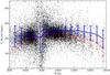 |
Fig. 3 Rotation speed as a function of R for bins with |z| < 200 pc, adopting a solar azimuthal speed of Vg, ⊙ = 250 km s-1 and an LSR azimuthal speed of Vc(R⊙,z = 0) = 238 km s-1. The dashed line is the weighted average of the bins without correction of systematic errors of the proper motion but taking into account the errors due to contamination of non-RCGs and including errors due to uncertainties in (U⊙,Vg, ⊙,W⊙). The solid line is the weighted average of the bins including the correction of systematic errors of the proper motion as explained in Sect. 5; error bars include statistical errors, uncertainties in (U⊙,Vg, ⊙,W⊙), errors due to contamination of non-RCGs and errors of systematic errors of proper motion (see Fig. 4). |
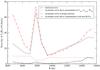 |
Fig. 4 Decomposition of the four sources of error, which sum quadratically to give the error bars plotted in the solid line of Fig. 3. |
5. Correcting systematic errors of the proper motions
Proper motions published by the PPMXL catalog have both statistical and systematic errors. The transmission of the statistical errors is taken into account in the previous steps; however, the systematic errors need to be accounted for as well because they are relatively high. In this subsection we calculate these systematic errors of the proper motions as a function of the Galactic coordinates.
Wu et al. (2011) analyzed the proper motions of 117 053 quasars within the PPMXL catalog. These sources are supposed to have null proper motions, because of their very large distances, so their average significant deviations from null proper motions can only stem from the systematic errors in PPMXL. Other authors (e.g., Bond et al. 2010, Sect. 2.3.1; Dong et al. 2011) have also used quasars to evaluate systematic errors of proper motions. Wu et al. (2011) found that the systematic errors depend on the coordinates, and they found no clear dependence with the magnitude or color of the sources. They also found that the quasars that are included in the 2MASS survey (13 520 sources) have a lower average systematic errors in the proper motion.
We used here the same subsample from 2MASS as was used in Sect. 4.4 of Wu et al. (2011): the 13 520 quasars. Because we also used sources that are both in PPMXL and the 2MASS survey, the systematic error in the proper motion of these quasars may well be applied to our sample of stars. Wu et al. (2011, Sect. 4.4) calculated an average μαcos(δ) = −1.4 mas/yr, μδ = −1.6 mas/yr. Here we extend their analysis of the PPMXL-2MASS quasars, using Galactic coordinates.
First, we confirm in this subsample of PPMXL-2MASS quasars the result given by Wu et al.
(2011) for the whole set of PPMXL quasars: we found
no significant correlation between proper motion and magnitude. In particular for the
K-magnitude,
a weighted linear fit of the proper motions gives us a
![Mathematical equation: \hbox{$\frac{{\rm d}[\mu _\ell \cos (b)]}{{\rm d}m_K}=+0.13\pm 0.10$}](/articles/aa/full_html/2014/03/aa23505-14/aa23505-14-eq121.png) mas/yr/mag,
mas/yr/mag, 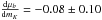 mas/yr/mag, which is
compatible with no dependence or a negligible one.
mas/yr/mag, which is
compatible with no dependence or a negligible one.
There is, however, a clear dependence of the quasars proper motions on position. In Fig. 5, we plot the median of the proper motion in bins of Δℓ = 15 deg., Δb = 15 deg. in Galactic coordinates for bins with more than 20 quasars.
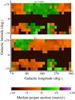 |
Fig. 5 Median of the proper motion of quasars included in the catalogs PPMXL and 2MASS. Bin size: 15 deg × 15 deg in Galactic coordinates. Green to violet indicates positive values; brown to orange indicates negative values; darkest colors indicate that there are fewer than 20 quasars in that bin, therefore no median was calculated. |
Regrettably, there are not enough quasars in the Galactic plane, the zone in which we are
interested. Instead, we carried out a linear weighted interpolation in both directions of
the map in Fig. 5, top panel, to derive the systematic
error Syst[μℓcosb] (ℓ,b)
with its corresponding statistical error. We took the error as the average error of the
pixel in the surrounding area. Then, we subtracted this systematic error from each of our
proper motions of our bins:  \label{corrsyst} , \end{eqnarray}](/articles/aa/full_html/2014/03/aa23505-14/aa23505-14-eq127.png) (9)and
thus derived a rotation speed corrected for systematic errors of proper motions. See Fig.
3 for the application in the z = 0 cases. To calculate of
the error bars, the statistical errors are reduced in the weighted average in proportion to
the root square of the number of data but the errors of Syst [μℓcosb] (ℓ,b)
are not, because they are common for large regions.
(9)and
thus derived a rotation speed corrected for systematic errors of proper motions. See Fig.
3 for the application in the z = 0 cases. To calculate of
the error bars, the statistical errors are reduced in the weighted average in proportion to
the root square of the number of data but the errors of Syst [μℓcosb] (ℓ,b)
are not, because they are common for large regions.
One may wonder about the advantage of including the correction of Eq. (9) if we still keep a systematic error in the error of Syst [μℓcosb] (ℓ,b). The answer is that the corrected values have an average null deviation, whereas the uncorrected proper motion does not. In Fig. 3 we illustrate how the correction shifts the rotation speed. See Fig. 4 for the distribution of the error bar sources.
6. Rotation curves
We are interested in the region R > 4 kpc, |z| < 2 kpc, which defines
the disk region. for R < 4 kpc we find the
non-axisymmetric structure with non-circular orbits of the long bar (López-Corredoira et al.
2007). for |z| > 2 kpc, the halo
becomes important and the stellar density of the disk is a factor ≲1/300 than at z = 0 (Bilir et al. 2008). Figure 6 shows
the rotation curves for different values of z including the correction of systematic errors in
the proper motions. Note that in these plots the error bars of the different bins are not
entirely independent because the systematic errors are not independent. We used
Vg, ⊙ = 250 ± 9
km s-1 (Schönrich
2012). If we had used the lowest value in the
recent literature of 200 km s-1 (McMillan & Binney 2010; Bhattacharjee et al. 2013; without any
error bar; at present, we are just interested to see the effect of the change of
Vg, ⊙ and we do not think
this is the correct value) and keeping R⊙ = 8 kpc (although, this should be lower
if we reduce Vg, ⊙; McMillan
& Binney 2010), we would have obtained
similar results, Fig. 7, which shows us that the
observed features in Vc(R) are not very
dependent on the value of Vg, ⊙. This is expected
because, according to Eq. (8), the rotation
curves derived with two different values of Vg, ⊙ are related by
 (10)The
error bars are dominated by the systematic errors due to contamination of non-RCGs (we have
assumed the most pessimistic scenario of a 20% contamination and that the proper motions of
these non-RCGs are all higher or lower than the median) and the systematic errors of the
proper motions derived using the QSOs reference, see Fig. 4. It can be appreciated that for the bins at R ≈ R⊙, the error bar is
much larger than others because we are observing the velocity of the stars with a small
angle with respect to the line of sight and consequently with most of its contribution in
the radial direction and a small one to the proper motions. This implies that
cos(φ + ℓ) in Eq. (8) is small; we derive at R ≈ R⊙ values of
Vc
10–35 km s-1 lower
than the assumed LSR circular speed, but they are perfectly consistent within the error
bars.
(10)The
error bars are dominated by the systematic errors due to contamination of non-RCGs (we have
assumed the most pessimistic scenario of a 20% contamination and that the proper motions of
these non-RCGs are all higher or lower than the median) and the systematic errors of the
proper motions derived using the QSOs reference, see Fig. 4. It can be appreciated that for the bins at R ≈ R⊙, the error bar is
much larger than others because we are observing the velocity of the stars with a small
angle with respect to the line of sight and consequently with most of its contribution in
the radial direction and a small one to the proper motions. This implies that
cos(φ + ℓ) in Eq. (8) is small; we derive at R ≈ R⊙ values of
Vc
10–35 km s-1 lower
than the assumed LSR circular speed, but they are perfectly consistent within the error
bars.
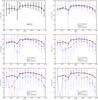 |
Fig. 6 Rotation speed derived from Eq. (8) as a function of R for different z, with Δz = 400 pc; correction of systematic errors of proper motions included; adopting a solar azimuthal speed of Vg, ⊙ = 250 km s-1 and a LSR azimuthal speed of Vc(R⊙,z = 0) = 238 km s-1. Error bars include statistical errors, uncertainties in (U⊙,Vg, ⊙,W⊙), and errors of the systematic errors of proper motion and contamination of non-RCGs (see Fig. 4 for the distribution of errors for z = 0). |
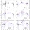 |
Fig. 7 Rotation speed derived from Eq. (8) as a function of R for different z, with Δz = 400 pc; correction of systematic errors of proper motions included; adopting a solar azimuthal speed of Vg, ⊙ = 200 km s-1 and an LSR azimuthal speed of Vc(R⊙,z = 0) = 188 km s-1. Error bars include statistical errors, uncertainties in (U⊙,Vg, ⊙,W⊙), and errors of the systematic errors of proper motion and contamination of non-RCGs. |
Considering Fig. 6, with Vg, ⊙ = 250 ± 9 km s-1, the following features are observed in these rotation curves:
-
In the Galactic plane (z = 0), we observe an almost constant rotation curve for R > R⊙ = 8 kpc, although with a slight slope for 13 < R(kpc)< 16. Because of the large error bars mostly due to uncertainties in the systematic effects, we cannot be sure that a flat rotation curve in this range is excluded. A decreasing rotation speed for the largest R of our range was also observed by other authors (Dias & Lépine 2005; Sofue et al. 2009). Nonetheless, for off-plane regions, this decreasing speed is more significant: for z ≳ 1 kpc we observe that highest rotation speed of ≈250 km s-1 is reached at R ≈ 10 kpc and then it decreases to values of ≈100 km s-1 at R ≈ 16 kpc, z = 2 kpc.
-
In the inner Galaxy, with R ≲ R⊙, given the huge error bars, we observe no systematic variation of the rotation curve with z. Our results are consistent with lower rotation speeds at higher z observed by other authors (Bond et al. 2010; Williams et al. 2013). for 13 < R (kpc) < 16, there is at z ≳ 1 kpc a lower rotation speed than at z = 0. On average for the results with Vg, ⊙ = 250 km s-1 and R⊙ < R < 2 R⊙,
![Mathematical equation: \begin{eqnarray} \frac{\partial V_{\rm c}(R,z)}{\partial |z|}=2.0+2.4~{\rm kpc}^{-1} \times (R-R_\odot) \\ -1.2~{\rm kpc}^{-2}\times [(R-R_\odot)]^2\ {\rm~km\,s}^{-1}/{\rm kpc}.\nonumber \end{eqnarray}](/articles/aa/full_html/2014/03/aa23505-14/aa23505-14-eq154.png) (11)
(11) -
We observe some asymmetry between the northern and southern Galactic hemisphere, with the southern one with higher rotations speeds, more significantly in the range 8 < R(kpc)< 13. However, again, this fact is observed in some bins with the error bars.
7. Dynamical consequences
The main challenge of our results is the low rotation velocity at the largest R, |z| within our range. Low rotation speed stars of ≈100 km s-1 were previously observed for the mean rotation velocity of some fraction of stars attributed to the thick-disk population at R ≈ R⊙ for low z (Fuchs et al. 1999) or at |z| ≈ 2 kpc (Gilmore et al. 2002). However, they were a minority of stars because the average rotation curve we observe for these coordinates is 150–200 km s-1, in agreement with Bond et al. (2010, Fig. 14). If the average rotation curve decreases to low values of Vc this means, if the result were correct, that the mass distribution declines almost in a Keplerian way (∝1/R). The rotation curve beyond 2 R⊙ was observed to possibly decline in Keplerian way in the Galactic plane (Honma & Sofue 1996), but not in off-plane regions like ours.
First we analyzed why our method leads to these low rotation speeds. The regions with R ≈ 16 kpc, |z| = 2 kpc are around the anticenter (ℓ = 180°) and | b| ≲ 14°, with apparent magnitude of the RCG stars mK ≈ 13.0; there are fewer bins than for other lower R (see Fig. 3). If we take, for instance, the region ℓ = 180°, b = + 7 (with Δℓ = 1°, Δb = 1°), we have 2802 stars from the PPMXL/2MASS catalog with mK < 14.0; for mK = 13.0 we determine a (J − K)0 = 0.81, and the corresponding RCGs with 12.8 < mK < 13.2, 0.62 < (J − K)0 < 1.01 are 138 stars. Assuming that all these stars are RCGs, this corresponds to an average distance of 7.8 kpc and an extinction of AK = 0.13, which is quite reasonable, and the selection of RCGs looks appropriate. We can see in Fig. 8 the color–magnitude diagram and the distribution of μℓ and μb of the selected RCGs. The median of the μℓcosb is 6.8 ± 1.6(95% C.L.; statistical only) ±1.8 (maximum systematic error due to 20% contamination) mas/yr. Certainly, as discussed in Sect. 3.1, some of the points in Fig. 8/middle might be contamination of local dwarfs or RGBBs. In Fig. 8 bottom panel, we see that these high proper motion cases, with either positive or negative values, are almost randomly distributed in colors, showing only a slight trend: redder colors give slightly higher proper motions in the direction of the Galactic longitude. A selection of RCGs in a narrower range of colors around (J − K)0 = 0.81 would not give a result significantly different from our 6.8 mas/yr. Now we correct for the systematic error in the proper motions: the bi-linear interpolation of the plot of Fig. 5 is Syst [μℓcosb] = 1.8 ± 0.9 mas/yr and hence (μℓcosb)corrected = 5.0 ± 1.8(stat.) ± 1.8 (syst.) mas/yr. At the attributed distance, this corresponds to a vℓ = 180 ± 70(stat.) ± 70(syst.) km s-1. In the anticenter (φ = 0, ℓ = 180°), following Eq. (8), vℓ = Vc − Vg, ⊙, therefore a significant departure from zero leads to a significant departure of the rotation speed with respect to the solar one. Are the systematic corrections of the proper motions are underestimated? It is possible, because interpolations/extrapolations are always dangerous, but in Fig. 5 there is not too much variation of Syst [μℓcosb] in the regions around our coordinate, Syst [μℓcosb] = 1.8 ± 0.9 mas/yr at ℓ = 180°, b = + 7° appears to be a reasonable interpolation. The five closest pixels in Fig. 5 give 2.1 ± 0.8 mas/yr at ℓ = 195°, b = + 15°; 1.1 ± 1.7 mas/yr at ℓ = 210°, b = + 15°; 1.2 ± 1.1 mas/yr at ℓ = 165°, b = + 30°; 1.5 ± 0.6 mas/yr at ℓ = 180°, b = + 30°; 0.6 ± 0.4 mas/yr at ℓ = 195°, b = + 30°, which are all close to the interpolated value of 1.8 ± 0.9. This is only for one bin, the represented points in Figs. 6 and 7 stand for a weighted average of several bins like this. To conclude, the origin of this strong decrease in rotation speeds is clear: the high values of (μℓcosb)corrected in off-plane regions of the anticenter. We obtain rotation speeds of Vc ≈ 100 km s-1 because we derive average (μℓcosb)corrected ≈ 4 mas/yr; the only possibility to make this number lower is considering that the systematic errors of 2–3 mas/yr are in the direction of reducing this proper motion toward 1–2 mas/yr, which would mean a Vc = 175 km s-1, which would agree better with expectations. At present, with the obtained results and the associated error bars, we cannot exclude this possibility.
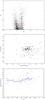 |
Fig. 8 Upper panel: RCG selection in a K vs. J − K color–magnitude diagram for the direction ℓ = 180°, b = 7°, mK,0 = 13.0, giving a maximum of counts within the RCG region at (J − K)0 = 0.81; the dashed rectangle represents the area where the RCGs are selected. Middle panel: proper motions of the selected RCG stars in the catalog PPMXL. Bottom panel: proper motion in the direction of Galactic longitude vs. color; the dashed line indicates the median of 20 points. |
A strong vertical gradient in Vc would mean that the disk contribution
is the most important one in the rotation curves for R ≤ 16 kpc. Since the radial
acceleration 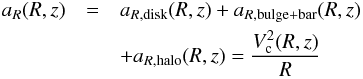 (12)is
very dependent on z for 13 < R(kpc)< 16, and
aR,bulge + bar and
aR,halo are almost
independent of z, we would deduce that the dominant component here is
aR,disk. The component of
mass distribution corresponding to the bulge+long bar is within R < 4
kpc and, although they are not spheroids, at Galactocentric distances of 13 < R(kpc) < 16 the acceleration
can be approximated by the monopolar Keplerian term:
(12)is
very dependent on z for 13 < R(kpc)< 16, and
aR,bulge + bar and
aR,halo are almost
independent of z, we would deduce that the dominant component here is
aR,disk. The component of
mass distribution corresponding to the bulge+long bar is within R < 4
kpc and, although they are not spheroids, at Galactocentric distances of 13 < R(kpc) < 16 the acceleration
can be approximated by the monopolar Keplerian term:
 (13)for
which
(13)for
which  (14)thus
the vertical gradient is negligible. Moreover Mbulge + bar ~ 2 × 10¹⁰ M⊙
(Sevenster et al. 1999; López-Corredoira et al. 2007), which is only a low ratio of the mass of the
Galaxy. For the halo, the total mass ratio is very high but most of contribution comes from
the outest Galaxy, much farther away than R = 16 kpc; a calculation of aR,halo using an oblate
spheroid of major axis a and vertical axis c < a with a
density distribution
(14)thus
the vertical gradient is negligible. Moreover Mbulge + bar ~ 2 × 10¹⁰ M⊙
(Sevenster et al. 1999; López-Corredoira et al. 2007), which is only a low ratio of the mass of the
Galaxy. For the halo, the total mass ratio is very high but most of contribution comes from
the outest Galaxy, much farther away than R = 16 kpc; a calculation of aR,halo using an oblate
spheroid of major axis a and vertical axis c < a with a
density distribution  (Battaglia et al. 2005) with s0 = 105 kpc and
 ,
we compute for
,
we compute for  that
that
 (15)a
negligible relative gradient in z; other models of the halo also give results on the
same order. Therefore, only a disk with a strong non-monopolar term could give a
contribution with a strong vertical gradient in Vc, and this would correspond to high
concentrations of mass in the outer disk. It was proved long time ago (Kuzmin 1952, 1955) that
there is no evidence for the presence of large amounts dark matter in the disk of the Galaxy
from observations in the solar neighborhood, and this is still confirmed today (Garbari et
al. 2012), but one might investigate whether amounts
of dark matter in the outer disk are possible. From the theoretical point of view at least,
it is a general solution for the observed rotation curves: Feng & Gallo (2011) showed that some mass distributions of the disk
alone might mimic the flat rotation curves of a galaxy (Mestel’s disk), without dark matter
halos, although these distributions are not realistic compared with the observed stellar
distribution (exponential).
(15)a
negligible relative gradient in z; other models of the halo also give results on the
same order. Therefore, only a disk with a strong non-monopolar term could give a
contribution with a strong vertical gradient in Vc, and this would correspond to high
concentrations of mass in the outer disk. It was proved long time ago (Kuzmin 1952, 1955) that
there is no evidence for the presence of large amounts dark matter in the disk of the Galaxy
from observations in the solar neighborhood, and this is still confirmed today (Garbari et
al. 2012), but one might investigate whether amounts
of dark matter in the outer disk are possible. From the theoretical point of view at least,
it is a general solution for the observed rotation curves: Feng & Gallo (2011) showed that some mass distributions of the disk
alone might mimic the flat rotation curves of a galaxy (Mestel’s disk), without dark matter
halos, although these distributions are not realistic compared with the observed stellar
distribution (exponential).
8. Summary and conclusions
Using only proper motions of sources identified as RCGs, we have derived the stellar rotation curve of the Galaxy in the range of Galactocentric radii of R = 4−16 kpc for different vertical shifts from the Galactic plane of z between –2 and +2 kpc. We obtained an almost flat rotation curve with a slight fall-off for higher values of R or |z|. The most puzzling result is the observed low average rotation speed at the outest and most off-plane cases, that is, at R ≈ 16 kpc and |z| ≈ 2, with less than the half of the rotation speed with respect to its value in the solar neighborhood region: on average for z = ± 2 kpc, Vc = 82 ± 5(stat.) ± 58(syst.) km s-1 (assuming the systematic errors at z = −2 kpc and z = + 2 kpc are independent, so they sum quadratically). If this speed is lower than 150 km s-1 (for Vg, ⊙ = 250 km s-1), it would have important consequences for the analysis of the dark matter distribution in the outer part of our Galaxy. Nevertheless, at present we cannot exclude that the strong vertical gradient in the rotation speed is caused only by a combined systematic error of proper motions and contamination with non-RCGs. The assumptions made here, such as the approximation of circular orbits, might also be relaxed in the outest part of the disk. More measurements of the proper motions at high R and z are warranted to confirm or refute these results.
Acknowledgments
Thanks are given to F. Garzón and the anonymous referee for helpful comments and suggestions to improve this paper. Thanks are given to Astrid Peter (language editor of A&A) for proof-reading of the text. The author was supported by the grant AYA2012-33211 of the Spanish Science Ministry. This work has used the data of PPMXL catalog (Roeser et al. 2010). Z.-Y. Wu has kindly provided the data corresponding to the results of the paper Wu et al. (2011).
References
- Aihara, H., de Prieto, C., An, D., et al. 2011, ApJS, 195, 26 [NASA ADS] [CrossRef] [Google Scholar]
- Battaglia, G., Helmi, A., Morrison, H., et al. 2005, MNRAS, 330, 35 [Google Scholar]
- Bhattacharjee, P., Chaudhury, S., & Kundu, S. 2013 [arXiv:1310.2659] [Google Scholar]
- Bilir, S., Cabrera-Lavers, A., Karaali, S., Ak, S., Yaz, E., & López-Corredoira, M. 2008, PASA, 25, 69 [NASA ADS] [CrossRef] [Google Scholar]
- Bobylev, V. V., Bajkova, A. T., & Stepanishchev, A. S. 2008, Astron. Lett., 34, 515 [NASA ADS] [CrossRef] [Google Scholar]
- Bond, N. A., Ivezić, Z., Sesar, B., et al. 2010, ApJ, 716, 1 [NASA ADS] [CrossRef] [Google Scholar]
- Bovy, J., Allen de Prieto, C., Beers, T. C., et al. 2012, ApJ, 759, 131 [NASA ADS] [CrossRef] [Google Scholar]
- Castellani, V., Chieffi, A., & Straniero, O. 1992, ApJS, 78, 517 [NASA ADS] [CrossRef] [Google Scholar]
- Cole, S., Norberg, P., Baugh, C., et al. 2001, MNRAS, 326, 255 [NASA ADS] [CrossRef] [Google Scholar]
- Dias, W. S., & Lépine, J. R. D. 2005, ApJ, 629, 825 [NASA ADS] [CrossRef] [Google Scholar]
- Dong, R., Gunn, J., Knapp, G., Rockosi, C., & Blanton, M. 2011, AJ, 142, 116 [NASA ADS] [CrossRef] [Google Scholar]
- Feng, J. Q., & Gallo, C. F. 2011, Res. Astron. Astrophys., 11, 1429 [NASA ADS] [CrossRef] [Google Scholar]
- Fuchs, B., Jahreiss, H., & Wielen, R. 1999, Ap&SS, 265, 175 [Google Scholar]
- Garbari, S., Liu, C., Read, J. I., & Lake, G. 2012, MNRAS, 425, 1445 [NASA ADS] [CrossRef] [Google Scholar]
- Gilmore, G., Wyse, R. F. G., & Norris, J. E. 2002, ApJ, 574, L39 [NASA ADS] [CrossRef] [Google Scholar]
- Golubov, O., Just, A., Bienaymé, O., et al. 2013, A&A, 557, A92 [NASA ADS] [CrossRef] [EDP Sciences] [Google Scholar]
- Honma, M., & Sofue, Y. 1996, PASJ, 48, L103 [NASA ADS] [CrossRef] [Google Scholar]
- Kuzmin, G. G. 1952, Tartu Astr. Obs. Publ. 32, 5 [NASA ADS] [Google Scholar]
- Kuzmin, G. G. 1955, Tartu Astr. Obs. Publ. 33, 3 [NASA ADS] [Google Scholar]
- Laney, C. D., Joner, M. D., & Pietrzyński, G. 2012, MNRAS, 419, 1637 [NASA ADS] [CrossRef] [Google Scholar]
- López-Corredoira, M., Cabrera-Lavers, A., Garzón, F., & Hammersley, P. L. 2002, A&A, 394, 883 [NASA ADS] [CrossRef] [EDP Sciences] [Google Scholar]
- López-Corredoira, M., & Betancort-Rijo, J. E. 2004, A&A, 416, 7 [NASA ADS] [Google Scholar]
- López-Corredoira, M., Cabrera-Lavers, A., Mahoney, T. J., et al. 2007, AJ, 133, 154 [NASA ADS] [CrossRef] [Google Scholar]
- Malkin, Z. M. 2013, Astron. Rep., 57, 128 [NASA ADS] [CrossRef] [Google Scholar]
- Marshall, D. J., Robin, A. C., Reylé, C., Schultheis, M., & Picaud, S. 2006, A&A, 453, 635 [NASA ADS] [CrossRef] [EDP Sciences] [Google Scholar]
- McMillan, P. J., & Binney, J. J. 2010, MNRAS, 402, 934 [NASA ADS] [CrossRef] [Google Scholar]
- Nataf, D. M., Gould, A., Fouqué, P., et al. 2013, ApJ, 769, 88 [NASA ADS] [CrossRef] [Google Scholar]
- Pietrzyński, G., Gieren, W., & Udalski, A. 2003, AJ, 125, 2494 [NASA ADS] [CrossRef] [Google Scholar]
- Reid, M. J., Menten, K. M., Brunthaler, A., et al. 2014, 783, 130 [Google Scholar]
- Reylé, C., Marshall, D. J., Robin, A. C., & Schultheis, M. 2009, A&A, 495, 819 [NASA ADS] [CrossRef] [EDP Sciences] [Google Scholar]
- Roeser, S., Demleitner, M., & Schilbach, E. 2010, AJ, 139, 2440 [NASA ADS] [CrossRef] [Google Scholar]
- Schönrich, R. 2012, MNRAS, 427, 274 [NASA ADS] [CrossRef] [Google Scholar]
- Sevenster, M. N., Prasenjit, S., Valls-Gabaud, D., & Fux, R. 1999, MNRAS, 307, 584 [NASA ADS] [CrossRef] [Google Scholar]
- Sofue, Y. 2011, PASJ, 63, 813 [NASA ADS] [CrossRef] [Google Scholar]
- Sofue, Y., Honma, M., & Omodaka, T. 2009, PASJ, 61, 227 [NASA ADS] [Google Scholar]
- Wegg, C., & Gerhard, O. E. 2013, MNRAS, 435, 1874 [Google Scholar]
- Williams, M. E. K., Steinmetz, M., Binney, J., et al. 2013, MNRAS, 436, 101 [NASA ADS] [CrossRef] [Google Scholar]
- Wu, Z.-Y., Ma, J., & Zhou, X. 2011, PASP, 12, 1313 [NASA ADS] [CrossRef] [Google Scholar]
- Yaz Gökçe, E., Bilir, S., Öztürkmen, N. D., et al. 2013, New Astron., 25, 19 [NASA ADS] [CrossRef] [Google Scholar]
All Figures
|
Fig. 1 Example of application of RCG selection from PPMXL survey in a K vs. J − K color–magnitude diagram. This case is for the direction ℓ = 125°, b = 2°, at one particular K-magnitude mK,0 = 13.0, giving a maximum of counts within RCG region at (J − K)0 = 1.25. The dashed rectangle represents the area where the RCGs are selected. |
| In the text | |
|
Fig. 2 Representation of kinematics of a star with respect to the Sun. |
| In the text | |
|
Fig. 3 Rotation speed as a function of R for bins with |z| < 200 pc, adopting a solar azimuthal speed of Vg, ⊙ = 250 km s-1 and an LSR azimuthal speed of Vc(R⊙,z = 0) = 238 km s-1. The dashed line is the weighted average of the bins without correction of systematic errors of the proper motion but taking into account the errors due to contamination of non-RCGs and including errors due to uncertainties in (U⊙,Vg, ⊙,W⊙). The solid line is the weighted average of the bins including the correction of systematic errors of the proper motion as explained in Sect. 5; error bars include statistical errors, uncertainties in (U⊙,Vg, ⊙,W⊙), errors due to contamination of non-RCGs and errors of systematic errors of proper motion (see Fig. 4). |
| In the text | |
|
Fig. 4 Decomposition of the four sources of error, which sum quadratically to give the error bars plotted in the solid line of Fig. 3. |
| In the text | |
|
Fig. 5 Median of the proper motion of quasars included in the catalogs PPMXL and 2MASS. Bin size: 15 deg × 15 deg in Galactic coordinates. Green to violet indicates positive values; brown to orange indicates negative values; darkest colors indicate that there are fewer than 20 quasars in that bin, therefore no median was calculated. |
| In the text | |
|
Fig. 6 Rotation speed derived from Eq. (8) as a function of R for different z, with Δz = 400 pc; correction of systematic errors of proper motions included; adopting a solar azimuthal speed of Vg, ⊙ = 250 km s-1 and a LSR azimuthal speed of Vc(R⊙,z = 0) = 238 km s-1. Error bars include statistical errors, uncertainties in (U⊙,Vg, ⊙,W⊙), and errors of the systematic errors of proper motion and contamination of non-RCGs (see Fig. 4 for the distribution of errors for z = 0). |
| In the text | |
|
Fig. 7 Rotation speed derived from Eq. (8) as a function of R for different z, with Δz = 400 pc; correction of systematic errors of proper motions included; adopting a solar azimuthal speed of Vg, ⊙ = 200 km s-1 and an LSR azimuthal speed of Vc(R⊙,z = 0) = 188 km s-1. Error bars include statistical errors, uncertainties in (U⊙,Vg, ⊙,W⊙), and errors of the systematic errors of proper motion and contamination of non-RCGs. |
| In the text | |
|
Fig. 8 Upper panel: RCG selection in a K vs. J − K color–magnitude diagram for the direction ℓ = 180°, b = 7°, mK,0 = 13.0, giving a maximum of counts within the RCG region at (J − K)0 = 0.81; the dashed rectangle represents the area where the RCGs are selected. Middle panel: proper motions of the selected RCG stars in the catalog PPMXL. Bottom panel: proper motion in the direction of Galactic longitude vs. color; the dashed line indicates the median of 20 points. |
| In the text | |
Current usage metrics show cumulative count of Article Views (full-text article views including HTML views, PDF and ePub downloads, according to the available data) and Abstracts Views on Vision4Press platform.
Data correspond to usage on the plateform after 2015. The current usage metrics is available 48-96 hours after online publication and is updated daily on week days.
Initial download of the metrics may take a while.