| Issue |
A&A
Volume 563, March 2014
|
|
|---|---|---|
| Article Number | A126 | |
| Number of page(s) | 10 | |
| Section | Celestial mechanics and astrometry | |
| DOI | https://doi.org/10.1051/0004-6361/201322649 | |
| Published online | 21 March 2014 | |
Mass estimates for visual binaries with incomplete orbits
Astrophysics Group, Blackett Laboratory, Imperial College London, Prince Consort
Road,
London
SW7 2AZ,
UK
e-mail:
l.lucy@imperial.ac.uk
Received:
11
September
2013
Accepted:
12
December
2013
The problem of estimating the total mass of a visual binary when its orbit is incomplete is treated with Bayesian methods. The posterior mean of a mass estimator is approximated by a triple integral over orbital period, orbital eccentricity and time of periastron. This reduction to 3D from the 7D space defined by the conventional Campbell parameters is achieved by adopting the Thiele-Innes elements and exploiting the linearity with respect to the four Thiele-Innes constants. The formalism is tested on synthetic observational data covering a variable fraction of a model binary’s orbit. The posterior mean of the mass estimator is numerically found to be unbiased when the data cover ≳40% of the orbit.
Key words: binaries: visual / stars: fundamental parameters / methods: statistical
© ESO, 2014
1. Introduction
Visual binaries are a fundamental source of data on stellar masses. An individual system
provides definitive data if it has a precise parallax ϖand a high
quality orbit yielding accurate values for the orbital period P and the semi-major axis
a. The total
mass of the binary in solar units is then given by Kepler’s third law
 (1)where
P is in years
and a and
ϖ are in
arcseconds. However, for many long-period binaries, the accumulated measurements do not
cover even one full orbit. The question therefore arises: can a high quality orbit be
derived from such incomplete data?
(1)where
P is in years
and a and
ϖ are in
arcseconds. However, for many long-period binaries, the accumulated measurements do not
cover even one full orbit. The question therefore arises: can a high quality orbit be
derived from such incomplete data?
In his classic monograph, Aitken (1918) gave the following answer: “in general, it is not worthwhile to compute the orbit of a double star until the observed arc not only exceeds 180°, but also defines both ends of the apparent ellipse”. Since the first observation will seldom coincide with either end point, Aitken’s criterion typically requires forb ≳ 0.75, where forb is the fraction of the orbit covered. Aitken also warns that when forb < 0.5 it will generally be possible to draw several very different ellipses each of which will satisfy the data about equally well.
Although definitive orbits are surely a prerequisite for definitive masses, Eggen (1967) noted that a3/P2 is often reasonably well determined even when a and P are not, a conclusion he reached by compiling data on systems with multiple computed orbits. He reports (Eggen 1962) that “In some cases there have been drastic revaluations of the period of a given pair but there is then a compensating change in a and the resulting values of a3/P2 suffer little alteration”. These same compensating changes in a and P also arise in the Monte Carlo search technique of Schaefer et al. (2006) − see their Fig. 13 for DF Tau.
Eggen’s examination of the historical record provides strong empirical evidence that useful masses can be obtained from incomplete orbits. But restricting the discussion to observed systems does not allow an assessment of the statistical properties of such mass estimates. Accordingly, in this paper, synthetic observations with forb < 1 are created for a binary with specified elements in order to test the accuracy of the derived total mass.
The problem of inferring masses from incomplete orbits will be particularly acute for data acquired by the Gaia satellite. Nurmi (2005) and Pourbaix (2011) estimate that ≳107 visual binaries will be discovered. Many of these will have periods longer than the five years planned for the mission, and their orbits could perhaps be analysed by the technique developed in this paper.
2. Bayesian estimation
As noted already by Aitken (1918), when an orbit is incomplete, several theoretical orbits will provide satisfactory fits. Two possible responses to this circumstance are: 1) scan parameter space to find the global minimum (e.g., Hartkopf et al. 1989) and assume that this orbit is the closest achievable approximation to the truth; or 2) scan parameter space to make a complete census of acceptable orbits and then compute an appropriate average of the individual mass determinations (e.g., Schaefer et al. 2006). However, a Bayesian approach is preferred here. Specifically, by scanning parameter space, the posterior means of the orbital elements or any function thereof can be computed without locating minima.
2.1. Orbital elements
The standard orbital elements describing a secondary’s motion relative to its primary are the Campbell elements θ = (P,T,e,a,i,ω,Ω). In addition to P and a previously defined, T is a time of periastron passage, e is the eccentricity, i is the inclination, ω is the longitude of periastron, and Ω is the position angle of the ascending node. However, for scanning parameter space, it is convenient to define an alternative to T. Noting that T can be replaced by T ± nP, where n is any integer, we choose T ∈ (0,P) and then define the alternative element τ = T/P ∈ (0,1).
The above Campbell elements are standard. But an alternative set, the Thiele-Innes elements (Appendix A), simplify Bayesian integrations. In these elements, the vector (a,i,ω,Ω) is replaced by ψ = (A,B,F,G), so that the 7-element vector of elements is now (φ,ψ), where φ = (P,e,τ).
Numerous authors have preferred the Thiele-Innes elements for conventional least-squares determinations of orbital parameters for both visual binaries and exoplanets (e.g., Hartkopf et al. 1989; Pourbaix et al. 2002; Schaefer et al. 2006; Casertano et al. 2008; Wright & Howard 2009). This paper argues that these elements are also advantageous for Bayesian estimation of orbital parameters.
2.2. Posterior mean
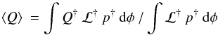
Let Q(θ) be a quantity whose value would
normally be computed after deriving a definitive orbit. But now in anticipation of there
being no single definitive orbit, we instead compute Q’s posterior mean, given
by  (2)Here
ℒ(φ,ψ|D) is the likelihood of the
elements (φ,ψ) given the data D, and p(φ,ψ) is
a probability density function (pdf) quantifying our prior beliefs or knowledge about the
orbital elements. In this problem, D comprises the secondary’s measured relative
Cartesian sky coordinates
(2)Here
ℒ(φ,ψ|D) is the likelihood of the
elements (φ,ψ) given the data D, and p(φ,ψ) is
a probability density function (pdf) quantifying our prior beliefs or knowledge about the
orbital elements. In this problem, D comprises the secondary’s measured relative
Cartesian sky coordinates  at
times tn.
at
times tn.
As remarked in Sect. 2.1, the Thiele-Innes elements simplify the integrations in Eq. (2).
For fixed φ = (P,e,τ), the family of
Keplerian orbits is linear in A,B,F,G. Accordingly, their least-squares values
 can be computed without iteration − see Sect. A.2. (Note that with normally-distributed errors the
least-squares solution is also the point of maximum likelihood (ML).)
can be computed without iteration − see Sect. A.2. (Note that with normally-distributed errors the
least-squares solution is also the point of maximum likelihood (ML).)
The second simplification concerns topology. When forb ≲ 0.5,
several orbits fit the data (Sect. 1). This implies severe topological complexity for
ℒ in the 7D (φ,ψ)-space. However, at
each point in φ-space, the 4D function
 is a quadrivariate normal distribution (Sect. A.3), which therefore has a single
peak at
is a quadrivariate normal distribution (Sect. A.3), which therefore has a single
peak at  ,
the point of ML.
,
the point of ML.
This topological simplification can be used in estimating the 7D integrals in Eq. (2). To
achieve this, we approximate the quadrivariate normal distribution by the delta function
 ,
so that
,
so that  (3)where
 (4)Thus, for each
point in φ-space, ℒ† is the value of ℒ at
(4)Thus, for each
point in φ-space, ℒ† is the value of ℒ at  ,
the ML point in ψ-space.
,
the ML point in ψ-space.
If we now replace ℒ in Eq.
(2) by the approximation given in Eq. (3) and integrate over ψ-space, we obtain
 (5)where the
superscript † indicates
evaluation at
(5)where the
superscript † indicates
evaluation at  as in Eq. (4).
On the assumption of normally-distributed measurement errors and with constants of
proportionality omitted, 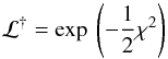 (6)where
 is the conventional goodness-fit criterion − see Eq. (A.5) − at φ = (P,e,τ).
In the statistics literature ℒ† is the profile likelihood (e.g., Severini 2000). This function is used in high energy physics for evaluating the significance of particle detections (e.g., Ranucci 2012).
2.3. Priors
In order to calculate the approximate posterior mean ⟨Q⟩ from Eq. (5),
 must be specified. Guided by common practice in Bayesian exoplanet detection (e.g., Ford
& Gregory 2007), we assume the elements to
have independent priors, so that p† is the
product of seven independent functions. The priors on the ψ elements are taken to be
uniform and so cancel between numerator and denominator in Eq. (5).
must be specified. Guided by common practice in Bayesian exoplanet detection (e.g., Ford
& Gregory 2007), we assume the elements to
have independent priors, so that p† is the
product of seven independent functions. The priors on the ψ elements are taken to be
uniform and so cancel between numerator and denominator in Eq. (5).
For the φ elements e and τ, the chosen priors are uniform in (0,1). For P, we adopt a Jeffreys prior − i.e., log P uniform in (log PL,log PU).
2.4. Numerical integration
The integrals in Eq. (5) are 3D as against 7D in Eq. (2). This reduction allows ⟨Q⟩ to be evaluated simply by computing the integrands at every point in a 3D grid and then summing. Without this reduction, a Markov chain Monte Carlo (MCMC) calculation would perhaps be required. Direct summation would, however, still be feasible if regions of negligible likelihood were efficiently excluded (Mikkelsen et al. 2012).
The integration domain in (log P,e,τ)-space is taken to be (log PL,log PU)
for log P,
and (0,1) for
both e and
τ. This
domain is partitioned into a 3D grid with constant steps for each variable. The quantity
Q is then
evaluated at the mid-points of the cells labelled (i,j,k) with
i ∈ (1,I), j ∈ (1,J),
k ∈ (1,K). The resulting formula for
the posterior mean is 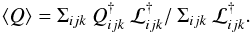 (7)The priors
adopted in Sect. 2.3 are implicitly incorporated since the cells are weighted equally.
(7)The priors
adopted in Sect. 2.3 are implicitly incorporated since the cells are weighted equally.
3. Calculation of ⟨Q⟩
In this section, the calculation of ⟨Q⟩ is described step-by-step.
3.1. Model binary
The model binary has the following Campbell elements:
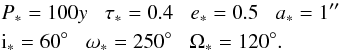 (8)From
Eqs. (A.1), the Thiele-Innes elements corresponding to the above values of a∗,i∗,ω∗,Ω∗
are
(8)From
Eqs. (A.1), the Thiele-Innes elements corresponding to the above values of a∗,i∗,ω∗,Ω∗
are  (9)
(9)
3.2. Synthetic data
Given these elements, the binary is “observed” at times
 (10)for n = 1,2,...,N,
so that the fraction forb of the orbit is uniformly sampled.
At each tn, the secondary’s
exact coordinates (xn,yn)
are computed from Eqs. (A.2)−(A.4). The measured positions are then
(10)for n = 1,2,...,N,
so that the fraction forb of the orbit is uniformly sampled.
At each tn, the secondary’s
exact coordinates (xn,yn)
are computed from Eqs. (A.2)−(A.4). The measured positions are then
 (11)where
each zG is a random Gaussian variate drawn from
(11)where
each zG is a random Gaussian variate drawn from
 and σ is the
standard error of unit weight. The vector (forb,N,σ) defines an
observing campaign.
and σ is the
standard error of unit weight. The vector (forb,N,σ) defines an
observing campaign.
Uniform sampling is here assumed for simplicity: it is not required by the Bayesian technique. Random sampling, the obvious alternative, is an inferior model for extant ground-based data on long-period binaries where typically an observation was made every observing season.
3.3. Calculation procedure
Given positions , a
posterior mean ⟨Q⟩ is computed as follows:
-
1)
The grid parameters I,J,K and PL,PU are specified.
-
2)
At each grid point, the vector φijk = (Pi,ej,τk) follows from the stepping procedure described in Sect. 2.4.
-
3)
Given φijk, the least-squares (ML) values of the Thiele-Innes elements
are computed from Eq. (A.7). -
4)
Given
 ,
the predicted positions (xn,yn)
are computed from Eqs. (A.2)−(A.4) and the resulting
,
the predicted positions (xn,yn)
are computed from Eqs. (A.2)−(A.4) and the resulting
 derived
from Eq. (A.5).
derived
from Eq. (A.5). -
5)
Given
, the
profile likelihood  is given by Eq. (6).
 -
6)
Given
,
the corresponding Campbell elements are computed from Eqs. (A.11)−(A.15) and used to evaluate
Qijk = Q(θijk).
-
7)
Given Qijk and
throughout the grid, ⟨Q⟩ is obtained from Eq. (7).
4. Feasible orbits
In this section, we exploit the scanning of parameter space required by the calculation of ⟨Q⟩ to relate the findings of Aitken and Eggen (Sect. 1) to the behaviour of ℒ†(φ|D).
4.1. A particular case
With orbital parameters from Eq. (8) and campaign parameters
 ,
synthetic data are calculated from Eq. (11). Then, with grid parameters PL = 0.7forbP∗,
PU = 300P∗,
I = 800,J = K = 200,
the values at all grid
points are determined as described in Sect. 3.3.
,
synthetic data are calculated from Eq. (11). Then, with grid parameters PL = 0.7forbP∗,
PU = 300P∗,
I = 800,J = K = 200,
the values at all grid
points are determined as described in Sect. 3.3.
If at grid point (i,j,k),
 (12)the elements
θijk are deemed to
represent a feasible orbit, and the ensemble of such orbits define the
feasible domain(s)
(12)the elements
θijk are deemed to
represent a feasible orbit, and the ensemble of such orbits define the
feasible domain(s)  in (log P,e,τ)-space.
In Fig. 1,
is projected onto the (log P,e) plane. Thus a filled circle appears at the
point (log Pi,ej)
if Eq. (12) is fulfilled for at least one τk. From this plot, we
see that for this poorly-observed incomplete orbit, there is an extended domain of
feasible orbits with P ranging from 40 to 5000y and e from 0.19 to >0.99.
Because
extends to the grid’s upper boundary at e = 1, a more general treatment would, in this
particular case, show that some parabolic and even hyperbolic orbits are feasible
− i.e., fit the data. By
restricting the analysis to elliptical orbits, unbound orbits are excluded. But this is
appropriate for the practical problem of concern: an incomplete observed orbit is highly
unlikely to be a close encounter of an unbound pair.
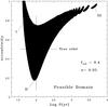 |
Fig. 1 Feasible domain |
In Fig. 2, the true orbit for this particular case
is plotted together with the measurements . Also
shown are three feasible orbits indicative of the range seen in Fig. 1. The Campbell elements of these are:
 (13)for
orbit I;
(13)for
orbit I; 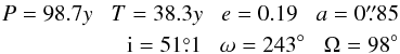 (14)for
orbit II; and
(14)for
orbit II; and 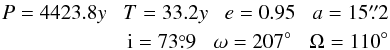 (15)for
orbit III.
(15)for
orbit III.
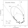 |
Fig. 2 Feasible orbits. Orbits I, II, III fit the measurements (filled circles) with an acceptable χ2. The bold curve is the true orbit with elements given in Eq. (8). |
Figure 2 illustrates and confirms Aitken’s warning (Sect. 1) that when forb < 0.5 several orbits will fit the data. Similar plots for real binaries are given by Schaefer et al. (2006).
Orbit III merits further comment. This orbit is nearly parabolic and has its periastron during the observing campaign. Thus, the observations were taken in time interval (0,40y) and periastron occurs at T = 33.2y. If this were the true orbit with P = 4423.8y, we would count ourselves fortunate to catch a periastron passage in such a short campaign. This is a generic feature of fitting orbits to short observed arcs: the orbit is not constrained when not observed and so can balloon out to large angular separations. This family of feasible orbits violate the Copernican Principle since the observer is inferred to be at a special epoch. Although this possibly justifies their exclusion, these orbits are retained in the calculation of posterior means.
4.2. Eggen’s effect
To investigate Eggen’s empirical discovery that even for poor orbits the ratio
a3/P2
is relatively reliable, the ensemble of feasible orbits plotted in Fig. 1 is now projected onto the (log P,log a) plane: Fig. 3. From this plot, we see a high density of points along
the line  (16)Thus, despite ranging in
period from 40 to
5000y, the
values of a3/P2
are relatively concentrated. This effect becomes even more striking with improved
campaigns having forb = 0.5 and 0.6 (see Fig. 3).
(16)Thus, despite ranging in
period from 40 to
5000y, the
values of a3/P2
are relatively concentrated. This effect becomes even more striking with improved
campaigns having forb = 0.5 and 0.6 (see Fig. 3).
These experiments indicate that with the chosen (N,σ), the feasible orbits are:
1): closely confined to (a∗,P∗) when forb ≳ 0.6;
2): dispersed widely in P but narrowly in a3/P2 when 0.5 ≳ forb ≳ 0.4;
3): dispersed widely in P and increasingly so in a3/P2 when forb ≲ 0.4.
These results provide strong theoretical support for Eggen’s discovery and for his use of the derived masses in studies of the mass-luminosity relation.
This confirmation derives from investigating the domain of high likelihood in (log P,e,τ)-space. Since this is the domain in which high weight is assigned to Q when its posterior mean is calculated, Eggen’s effect is evidently incorporated when this formalism is used to estimate the binary’s mass. Accordingly, Fig. 3 implies that we can anticipate useful results in this standard case provided that forb ≳ 0.4.
The explanation of Eggen’s effect is that as soon as secondary’s relative motion reveals a significant departure from rectilinear motion (forb ≪ 1) then acceleration has been detected and this is ∝ (ℳ1 + ℳ2) ∝ a3/P2. As forb increases, the uncertainty due to orientation factors decreases and so a3/P2 is well-determined before the orbit is complete − see also Heintz (1978) and Schaefer et al. (2006).
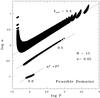 |
Fig. 3 Eggen’s effect. Feasible domains |

In addition to the linear trends, Fig. 3 shows a
dramatic increase in the volume of
as forb decreases from 0.6 to 0.4, supporting Aitken’s warning about the
onset of multiple acceptable orbits. Note that this increase in volume is a generic effect
that is not sensitive to the choice of 0.05 in Eq. (12).
This section has shown that the insights of Aitken and Eggen from 50−100 years ago find their modern explanation in how the topology of the likelihood function ℒ†(φ|D) responds to changes in the observational data D.
5. Mass estimates
The analysis of Sects. 2 and 3 is now applied to simulated partial orbits for the standard visual binary. Results with variations of e and i are reported in Appendix C.
5.1. Mass estimator
At the grid point (i,j,k), the φ elements are
(Pi,ej,τk),
and the
elements are the least-squares values  .
From the latter, the remaining Campbell elements
.
From the latter, the remaining Campbell elements  are computed as described in Sect. A.4, and we denote this semi-major axis as
âijk.
are computed as described in Sect. A.4, and we denote this semi-major axis as
âijk.
Now if ℳ∗ is the
true total mass of the model binary with orbit defined by Eq. (8), the inferred mass with
the orbit corresponding to the point (i,j,k) is
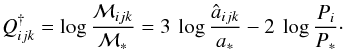
 (17)The natural choice for
the mass variable to be substituted in Eq. (7) is therefore ℳijk. However,
numerical experiments demonstrate that ⟨log ℳ⟩ is more accurate than log ⟨ℳ⟩. Accordingly, we take
(17)The natural choice for
the mass variable to be substituted in Eq. (7) is therefore ℳijk. However,
numerical experiments demonstrate that ⟨log ℳ⟩ is more accurate than log ⟨ℳ⟩. Accordingly, we take
 (18)Exploiting the
freedom to set ℳ∗ = 1, we now substitute Eq. (18) into Eq. (7) to obtain
the posterior mean ⟨log ℳ⟩,
where ℳ is the ratio of the
inferred to the exact mass. Thus, if the exact mass is recovered, then ⟨log ℳ⟩ = 0.
(18)Exploiting the
freedom to set ℳ∗ = 1, we now substitute Eq. (18) into Eq. (7) to obtain
the posterior mean ⟨log ℳ⟩,
where ℳ is the ratio of the
inferred to the exact mass. Thus, if the exact mass is recovered, then ⟨log ℳ⟩ = 0.
5.2. Numerical experiments
In these experiments, the true orbit is again given by Eq. (8). In the first sequence of
campaigns, N = 15 and  as in Sect. 4, but now forb is treated as a continuous
variable, thus investigating the deterioration of mass estimates as forb → 0. Note
that when forb changes so does the seed for the
random number generator. The pattern of Gaussian variates in Eq. (11) is therefore never
repeated.
as in Sect. 4, but now forb is treated as a continuous
variable, thus investigating the deterioration of mass estimates as forb → 0. Note
that when forb changes so does the seed for the
random number generator. The pattern of Gaussian variates in Eq. (11) is therefore never
repeated.
With steps of 0.01 in forb, the values of ⟨log ℳ⟩ are plotted in Fig. 4. We see that for forb ≳ 0.40, the mass estimates scatter about the exact value ℳ = 1 with errors <0.1 dex. However, for forb ≲ 0.40, the scatter increases sharply, with the error first exceeding 0.1 dex at forb = 0.38. These results are consistent with the implications of Fig. 3.
Accuracy should improve with more data or data of higher precision − i.e, with decreasing precision parameter
 .
This is investigated by reducing σ from
.
This is investigated by reducing σ from  to
to  while keeping N = 15. This second sequence is plotted in Fig. 4 as filled circles. As expected, the quality of the
estimates dramatically inproves: the errors are <0.012 dex for forb ≥ 0.36, but
increase sharply thereafter. Note that decreasing η by a factor of 10 has
only slightly extended the domain of reliable solutions − the error first exceeds 0.1 dex at
forb = 0.34.
while keeping N = 15. This second sequence is plotted in Fig. 4 as filled circles. As expected, the quality of the
estimates dramatically inproves: the errors are <0.012 dex for forb ≥ 0.36, but
increase sharply thereafter. Note that decreasing η by a factor of 10 has
only slightly extended the domain of reliable solutions − the error first exceeds 0.1 dex at
forb = 0.34.
These experiments demonstrate that ⟨log ℳ⟩ provides a seemingly unbiased estimate of a visual binary’s total mass even when standard orbit fitting generates multiple acceptable solutions with a large range of orbital periods.
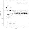 |
Fig. 4 Mass estimator. The posterior mean of log ℳ is plotted against forb. The
campaigns with |

5.3. Posterior pdf of log ℳ
For a real binary with an incomplete orbit, forb is unknown. Moreover, perhaps counterintuitively, it cannot even be reliably estimated. Figure 2 and Eqs. (13)−(15) illustrate this: for orbit I, forb = 0.85; for orbit II, forb = 0.41; and for orbit III, forb = 0.009, as against the true value 0.4. It follows that an investigator cannot judge the accuracy of ⟨log ℳ⟩ from an estimate of forb. Instead, the posterior pdf of log ℳ should be derived and credible intervals computed.
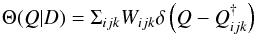
Inspection of Eq. (7) shows that the implied approximation to the posterior pdf is
 (19)where
δ is the
delta function, and
(19)where
δ is the
delta function, and  (20)From these
formulae, we immediately find
(20)From these
formulae, we immediately find 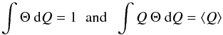 (21)where ⟨Q⟩ is the approximation
given by Eq. (7).
(21)where ⟨Q⟩ is the approximation
given by Eq. (7).
A histogram representation of the pdf Θ(log ℳ|D) is obtained by convolving Eq. (19) with a top-hat function. Examples are plotted in Fig. 5 for forb = 0.4 and 0.5. These show the loss of precision with decreasing forb that was expected from Fig. 3 and seen in Fig. 4.
The equivalent of 1σ Gaussian error bars can be computed from these
pdf’s by finding the equal area tails that together comprise 31.7% of the probability. Thus, we find
 for forb = 0.5 and
 for forb = 0.4.
Because the pdf Θ(log ℳ|D) is approximately Gaussian (see Fig.
5) the above error bars can with sufficient
accuracy be replaced by the standard deviation of the pdf, given by
 (22)This formula gives
slog ℳ = 0.019 and 0.085 for forb = 0.5 and
0.4, respectively.
Evidently, the dramatic loss in precision when the orbital coverage is insufficient is
apparent from slog ℳ even without knowing
forb.
(22)This formula gives
slog ℳ = 0.019 and 0.085 for forb = 0.5 and
0.4, respectively.
Evidently, the dramatic loss in precision when the orbital coverage is insufficient is
apparent from slog ℳ even without knowing
forb.
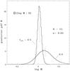 |
Fig. 5 Posterior pdf Θ(log ℳ|D) for forb = 0.4
and 0.5 both with
|

5.4. Bias
For forb ≳ 0.4, Fig. 4 shows no evidence that the estimator ⟨log ℳ⟩ is biased. But for forb ≲ 0.4, any bias is obscured by the dramatic increase in scatter. Accordingly, since quantifying the onset of bias is of interest in understanding the limits of this Bayesian approach, further calculations are now reported.
In order to beat down the noise, the campaigns with
 are repeated n = 100 times for selected values of forb. The
average and variance
are repeated n = 100 times for selected values of forb. The
average and variance 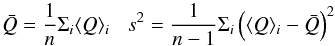 (23)of
the ⟨Q⟩ i are computed,
so that the resulting estimate is
(23)of
the ⟨Q⟩ i are computed,
so that the resulting estimate is  ,
and this indicates bias if it differs significantly from the exact value of
Q.
,
and this indicates bias if it differs significantly from the exact value of
Q.
Figure 6 presents evidence of bias for the estimator ⟨log (ℳ)⟩. The average values of ⟨log (ℳ)⟩ and their standard deviations from 100 independent realisations of the orbits are plotted for forb = 0.30(0.05)0.95. There is no evidence of bias for forb ≥ 0.6, but strong evidence for forb ≤ 0.4 where the displacements are >3.5s. Similar plots are given in Appendix B for the posterior means of the Campbell elements.
The onset of bias coincides with the onset of scatter (see Fig. 4) at which point accurate mass determinations are no longer possible.
Nevertheless, from a technical standpoint, it is of interest to understand the origin of
bias. Comparison of Figs. 2, 3, and 6 shows that the onset of bias corresponds to the
dramatic increase in the volume of ,
and this implies that the choice of priors becomes increasingly important. Accordingly,
since the expansion of
brings in orbits of high eccentricity (Fig. 2), we
might seek to penalize such orbits via the prior on e. But this would be an
ad hoc fix for this particular model binary. A
fundamental solution probably invokes the Copernican Principle (Sect. 4.1) to reduce the
weight assigned to highly eccentric orbits.
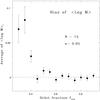 |
Fig. 6 Bias of the posterior mean ⟨log (ℳ)⟩. The averages and standard errors from Eq. (23)
plotted against forb with
|
5.5. Coverage fractions
When the estimate of a parameter derived by least-squares analysis is reported as
 ,
we automatically interpret this as an assertion that there is a 68.3% probability that the true answer lies
in the interval
,
we automatically interpret this as an assertion that there is a 68.3% probability that the true answer lies
in the interval  .
Implicit in this interpretation, however, are the following assumptions: 1)
normally-distributed measurement errors; 2) the validity of the linearization used in
deriving the normal equations; and 3) that the number of data points N greatly exceeds
M, the
number of parameters estimated. If one or more these assumptions does not hold then the
above interval’s coverage fraction will differ from 0.683.
.
Implicit in this interpretation, however, are the following assumptions: 1)
normally-distributed measurement errors; 2) the validity of the linearization used in
deriving the normal equations; and 3) that the number of data points N greatly exceeds
M, the
number of parameters estimated. If one or more these assumptions does not hold then the
above interval’s coverage fraction will differ from 0.683.
In Bayesian statistics, credibility intervals derived from the posterior pdf replace the confidence intervals of frequentist statistics, and the different meanings of these intervals has been topic of much discussion in the statistical literature over many years. One approach to reconciling this aspect of the Bayesian-frequentist debate is that of calibrated Bayes (e.g., Dawid 1982; Little 2006): a credible interval is well-calibrated if the enclosed probability matches the fraction of times that it contains the true value.
In order to test whether credible intervals calculated with this formalism for visual
binaries are well-calibrated, 1000 independent realizations of two campaigns with
 have been analysed, one with forb = 0.60, the other with
forb = 0.95. For each realization, we
check if Qexact is in the intervals (⟨Q⟩ −msQ, ⟨Q⟩ + msQ)
for m = 1,2, where ⟨Q⟩ is given by Eq. (7)
and sQ by Eq. (22).
have been analysed, one with forb = 0.60, the other with
forb = 0.95. For each realization, we
check if Qexact is in the intervals (⟨Q⟩ −msQ, ⟨Q⟩ + msQ)
for m = 1,2, where ⟨Q⟩ is given by Eq. (7)
and sQ by Eq. (22).
The results of this exercise are in Table 1. The first row gives the desired fraction ℰ(f)− i.e., the fraction expected for an ideal frequentist analysis. The remaining rows give the results for the posterior means of the Campbell elements and log ℳ.
Inspection of these results shows that the coverage is close to ideal for the φ elements P,e,τ. Accordingly, their credible intervals are well-calibrated. However, for the remaining elements and for log ℳ, the error bars are too small by factors of 1.1−2.1 at 1σ and 1.1−1.6 at 2σ. These error bars could of course be calibrated from such simulations. However, these shortfalls occur for the elements that were replaced by the Thiele-Innes constants and thus had the widths of their posterior pdfs reduced by the delta function approximation in Eq. (3). Further research based on the analytical formulae of Sect. A.3 may alleviate or eliminate this problem.
Coverage fractions f from 1000 trials.
6. Conclusion
The aim of this paper has been to apply Bayesian methods to a problem that dates back a century or more, namely how to estimate the total mass of a visual binary that has a measured parallax but an incomplete orbit. This problem has previously been effectively treated by Schaefer et al. (2006) with a heuristic Monte Carlo search technique. In contrast, the Bayesian approach has a firm theoretical foundation and is, moreover, now the preferred methodology in many areas of astronomy, notably in cosmology (e.g., Liddle 2009) and in the discovery and characterization of the orbits of exoplanets (e.g., Ford & Gregory 2007).
A further merit of Bayesian estimation for visual binaries is that only triple integrals need to be evaluated when the quadrivariate normal distribution of the Thiele-Innes constants (Sect. A.3) is approximated by a delta function (Sect. 2.2). The use of this approximation might be expected to introduce systematic errors in the derived elements. However, the failure to detect bias when forb ≳ 0.5 (Sect. 5.4, Appendix B) demonstrates that such errors are not of practical concern.
In Sect. 1, the possible application to binaries discovered by Gaia was mentioned. However, the simulations reported in this paper relate to ground-based data where two sky coordinates are measured. In contrast, the scanning mode of Gaia will provide ~70 high precision one dimensional measurements of a secondary’s displacement (e.g., Pourbaix 2002; Lattanzi et al. 2000). Simulations of a model binary observed in this manner are required to demonstrate the merits of this Bayesian approach for Gaia.
Acknowledgments
I thank D.J. Mortlock for a helpful discussion on nuisance parameters and profile likelihoods. I am obliged to the referee for suggestions that improved the paper.
References
- Aitken, R. G. 1918, The Binary Stars (New York: D. C. McMurtrie), 92 [Google Scholar]
- Casertano, S., Lattanzi, M. G., Sozzetti, A., et al. 2008, A&A, 48, 699 [NASA ADS] [CrossRef] [EDP Sciences] [Google Scholar]
- Dawid, A. P. 1982, Journal of the American Statistical Association, 77, 605 [Google Scholar]
- Eggen, O. J. 1962, QJRAS, 3, 259 [NASA ADS] [Google Scholar]
- Eggen, O. J. 1967, ARA&A, 5, 105 [NASA ADS] [CrossRef] [Google Scholar]
- Ford, E. B., & Gregory, P. C. 2007, ASPC, 371, 189 [Google Scholar]
- Hartkopf, W. I., McAlister, H. A., & Franz, O. G. 1989, AJ, 98, 1014 [NASA ADS] [CrossRef] [Google Scholar]
- Heintz, W. D. 1978, Double Stars (Reidel, Dordrecht), 63 [Google Scholar]
- Lattanzi, M. G., Spagna, A., Sozzetti, A., & Casertano, S. 2000, MNRAS, 317, 211 [NASA ADS] [CrossRef] [Google Scholar]
- Liddle, A. R. 2009, Ann. Rev. Nucl. Particle Sci., 59, 95 [NASA ADS] [CrossRef] [Google Scholar]
- Little, R. 2006, The American Statistician, 60, 1 [CrossRef] [Google Scholar]
- Mikkelsen, K., Nss, S. K., & Eriksen, H. K. 2012, ApJ, submitted [Google Scholar]
- Nurmi, P. 2005, ESA SP, 576, 463 [NASA ADS] [Google Scholar]
- Pourbaix, D. 2002, A&A, 385, 686 [NASA ADS] [CrossRef] [EDP Sciences] [Google Scholar]
- Pourbaix, D. 2011, AIP Conf. Proc., 1346, 122 [Google Scholar]
- Ranucci, G. 2012, Nucl. Instr. Meth. Phys. Res. A, 661, 77 [NASA ADS] [CrossRef] [Google Scholar]
- Schaefer, G. H., Simon, M., Beck, T. L., Nelan, E., & Prato, L. 2006, AJ, 132, 2618 [NASA ADS] [CrossRef] [Google Scholar]
- Severini, T. A. 2000, Likelihood Methods in Statistics (Oxford: OUP) [Google Scholar]
- Wright, J. T., & Howard, A. W. 2009, ApJS, 182, 205 [NASA ADS] [CrossRef] [Google Scholar]
Appendix A: Thiele-Innes elements
In this Appendix, a concise self-contained account of the Thiele-Innes elements is presented − see also Wright & Howard (2009) and Hartkopf et al. (1989). The explicit least-squares formulae for A,B,F,G and for their variances and covariances are new − Eqs. (A.7), (A.9), (A.10).
Appendix A.1: Definitions
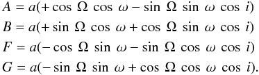
The Thiele-Innes constants A,B,F,G are defined in terms of four of the Campbell elements. Specifically,
Given these constants, the coordinates (x,y) of the secondary relative to the primary at
time t are
 (A.2)where
 (A.3)and
E(t), the eccentric anomaly, is
given by Kepler’s equation
(A.3)and
E(t), the eccentric anomaly, is
given by Kepler’s equation  (A.4)
(A.4)
Appendix A.2: Least-squares estimates
On the assumption that P,e,T are known, the determination of the four
Thiele-Innes elements is a straightforward problem of fitting a linear
model to the data. If the observed position at tn is
, then
estimates for A,B,F,G may be obtained by minimizing
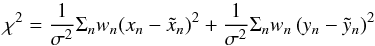 (A.5)where
(xn,yn)
is the theoretical position given by Eq. (A.2). Here wn is the weight of the
nth
observation and σ is the standard error of a measurement of unit
weight.
(A.5)where
(xn,yn)
is the theoretical position given by Eq. (A.2). Here wn is the weight of the
nth
observation and σ is the standard error of a measurement of unit
weight.
This least-squares problem can be solved without iteration since x and y are linear in A,B,F,G. Moreover, the first term in Eq. (A.5) depends only on the pair (A,F) and the second term only on (B,G). Accordingly, the estimates for A,F are obtained by minimizing the first term in Eq. (A.5) and those for B,G by minimizing the second term. Thus, the problem reduces to solving two independent pairs of linear equations, each with two unknowns.
To simplify the resulting formulae, we define the following quantities
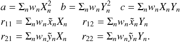 (A.6)The
least-squares estimates for the Thiele-Innes constants are then
(A.6)The
least-squares estimates for the Thiele-Innes constants are then
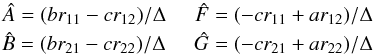 (A.7)where
Δ = ab − c2.
(A.7)where
Δ = ab − c2.
The above analysis is readily generalized to allow
 to have different weights
  . In the
formulae for
. In the
formulae for  ,
the quantities a,b,c,r11,r12
are evaluated with
,
the quantities a,b,c,r11,r12
are evaluated with  .
Correspondingly, in the formulae for
.
Correspondingly, in the formulae for  ,
the quantities a,b,c,r21,r22
are evaluated with
,
the quantities a,b,c,r21,r22
are evaluated with  .
.
Appendix A.3: Covariance matrix
The two sets of normal equations solved above for
and
have the same matrix of coefficients and therefore the same inverse. These are
 (A.8)From the coefficients
of the covariance matrix M-1, we derive
(A.8)From the coefficients
of the covariance matrix M-1, we derive
 (A.9)and
 (A.10)The covariances of
other pairings of A,B,F,G are zero. Note that these results apply for
fixed P,e,T.
(A.10)The covariances of
other pairings of A,B,F,G are zero. Note that these results apply for
fixed P,e,T.
The above analysis shows that (A,F) have a bivariate normal distribution
centred on  with variances and covariance from Eqs. (A.9) and (A.10) − and correspondingly for the pair
(B,G).
Accordingly, the pdf p(A,B,F,G|φ)
is a quadrivariate normal distribution centred on
with variances and covariance from Eqs. (A.9) and (A.10) − and correspondingly for the pair
(B,G).
Accordingly, the pdf p(A,B,F,G|φ)
is a quadrivariate normal distribution centred on
 .
This explicit derivation of p(ψ|φ) could
be used to replace the delta function in Eq. (3).
.
This explicit derivation of p(ψ|φ) could
be used to replace the delta function in Eq. (3).
Appendix A.4: Campbell elements
Having derived the least-squares values of A,B,F,G from Eqs. (A.7), we must invert the
transformation given by Eq. (A.1). The angle ω + Ω is the solution of the equation
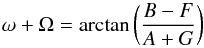 (A.11)such
that sin(ω + Ω) has the same sign as B − F.
Similarly, ω − Ω is the solution of the equation
(A.11)such
that sin(ω + Ω) has the same sign as B − F.
Similarly, ω − Ω is the solution of the equation
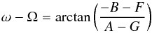 (A.12)such
that sin(ω − Ω) has the same sign as −B − F.
This pair of equations can be solved for ω and Ω. But Ω
may violate the convention that Ω ∈ (0,π). Accordingly, if Ω < 0, we set
Ω = Ω + π
and ω = ω + π. But
if Ω > π, we set
Ω = Ω − π
and ω = ω − π.
(A.12)such
that sin(ω − Ω) has the same sign as −B − F.
This pair of equations can be solved for ω and Ω. But Ω
may violate the convention that Ω ∈ (0,π). Accordingly, if Ω < 0, we set
Ω = Ω + π
and ω = ω + π. But
if Ω > π, we set
Ω = Ω − π
and ω = ω − π.
If we now define 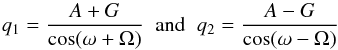 (A.13)then
the inclination is
(A.13)then
the inclination is  (A.14)and
the semi-major axis is
(A.14)and
the semi-major axis is  (A.15)
Appendix B: Bias of posterior means
The numerical search for bias reported in Sect. 5.4 also included the Campbell elements. The results are plotted in Figs. B.1−B.7. The behaviour revealed by these plots is broadly similar to that seen in Fig. 6 except that for some elements bias is evident at somewhat larger forb. Thus biases >3s occur at forb = 0.5 for ⟨log P⟩ , ⟨log a⟩ , ⟨τ⟩ and ⟨e⟩.
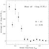 |
Fig. B.1 Bias of the posterior mean ⟨log (P/P∗)⟩.
The averages and standard errors from Eq. (23) are plotted against forb with
|
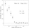 |
Fig. B.2 Bias of the posterior mean ⟨log (a/a∗)⟩.
The averages and standard errors from Eq. (23) are plotted against forb with
|
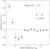 |
Fig. B.3 Bias of the posterior mean ⟨τ⟩. The averages and standard errors from
Eq. (23) are plotted against forb with
|
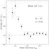 |
Fig. B.4 Bias of the posterior mean ⟨e⟩. The averages and standard errors from
Eq. (23) are plotted against forb with
|
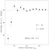 |
Fig. B.5 Bias of the posterior mean ⟨i⟩. The averages and standard errors from Eq. (23) are
plotted against forb with
|
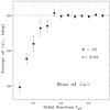 |
Fig. B.6 Bias of the posterior mean ⟨ω⟩. The averages and standard errors from
Eq. (23) are plotted against forb with
|
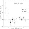 |
Fig. B.7 Bias of the posterior mean ⟨Ω⟩. The averages and standard errors from Eq. (23) are
plotted against forb with
|
Appendix C: Variation of parameters
In this Appendix, posterior means are computed when selected orbital parameters are
varied from those of the standard model; see Eq. (8). Specifically, in one sequence
e = 0.00(0.19)0.95, and in a second sequence
i = 0°(18°)90°, with, in
each case, the other elements as in Eq. (8). For both sequences, the campaign parameters
are  ,
and each orbit is computed with a different random number seed. The orbits are poor and
incomplete but forb is in the domain (forb ≳ 0.6)
where bias due to priors is negligible; see Sect. 5.4 and Appendix B.
,
and each orbit is computed with a different random number seed. The orbits are poor and
incomplete but forb is in the domain (forb ≳ 0.6)
where bias due to priors is negligible; see Sect. 5.4 and Appendix B.
Sequence with varying eccentricity e.
Sequence with varying inclination i.
Results for the e-sequence are in Table C.1. Aspects to note are as follows: The solution for e = 0 has large error bars for ⟨ω⟩ and ⟨τ⟩. These arise because ω and τ = T/P become meaningless and indeterminate as e → 0 - i.e., for a circular orbit. Also since e is non-negative, ⟨e⟩ is positively-biased when the true value is e = 0. Despite these issues, an accurate mass is obtained.
At the other extreme of highly elliptical orbits, Table C.1 reveals large error bars for all elements except ⟨e⟩.
Results for the i-sequence are in Table C.2. Aspects to note are as follows: The solution i = 0°− i.e., a face-on orbit - has large error bars for ω and Ω. From Eqs. (A.1), we see that when i = 0°, A = G = acos(ω + Ω) and B = −F = asin(ω + Ω). Accordingly, for an exactly face-on orbit, the difference ω − Ω is indeterminate, and the error bars on ω and Ω reflect this. Nevertheless, the mass determination is accurate.
As was the case for ⟨e⟩, the quantity ⟨i⟩ is postively-biased
since i is
non-negative. The expected magnitude of this bias can be computed independently of the
Bayesian code. If we assume that P,e,τ have the values given in Eq. (8), then the
least-squares fit to a synthetic orbit with i = 0 is derived with Eqs. (A.7) and then the corresponding Campbell
elements a,i,ω,Ω obtained with Eqs.
(A.11)−(A.15). With the
chosen campaign parameters, n = 1000 repetitions of this calculation gives the
average value  ,
consistent with
,
consistent with  in Table C.2. When σ is reduced to
as in Sect. 5.2,
in Table C.2. When σ is reduced to
as in Sect. 5.2,  .
Thus, as expected, the bias of i decreases with improved data.
.
Thus, as expected, the bias of i decreases with improved data.
A further point of note in the i-sequence is that the standard error of ⟨Ω⟩ is much smaller than that of
⟨ω⟩ when
i = 90°− i.e., an edge-on orbit. Although the error
bars of these elements are somewhat underestimated (Sect. 5.5), this is a real effect.
From Eqs. (A.1) and (A,2), it follows that the exact edge-on orbit obeys the equation
y/x = tanΩ, so
that Ω is determined by the
slope of the straight line fitted to .
The Bayesian code does not formally make such a fit, but this mathematical aspect is
implicit.
All Tables
All Figures
|
Fig. 1 Feasible domain |
| In the text | |
|
Fig. 2 Feasible orbits. Orbits I, II, III fit the measurements (filled circles) with an acceptable χ2. The bold curve is the true orbit with elements given in Eq. (8). |
| In the text | |
|
Fig. 3 Eggen’s effect. Feasible domains |
| In the text | |
|
Fig. 4 Mass estimator. The posterior mean of log ℳ is plotted against forb. The
campaigns with |
| In the text | |
|
Fig. 5 Posterior pdf Θ(log ℳ|D) for forb = 0.4
and 0.5 both with
|
| In the text | |
|
Fig. 6 Bias of the posterior mean ⟨log (ℳ)⟩. The averages and standard errors from Eq. (23)
plotted against forb with
|
| In the text | |
|
Fig. B.1 Bias of the posterior mean ⟨log (P/P∗)⟩.
The averages and standard errors from Eq. (23) are plotted against forb with
|
| In the text | |
|
Fig. B.2 Bias of the posterior mean ⟨log (a/a∗)⟩.
The averages and standard errors from Eq. (23) are plotted against forb with
|
| In the text | |
|
Fig. B.3 Bias of the posterior mean ⟨τ⟩. The averages and standard errors from
Eq. (23) are plotted against forb with
|
| In the text | |
|
Fig. B.4 Bias of the posterior mean ⟨e⟩. The averages and standard errors from
Eq. (23) are plotted against forb with
|
| In the text | |
|
Fig. B.5 Bias of the posterior mean ⟨i⟩. The averages and standard errors from Eq. (23) are
plotted against forb with
|
| In the text | |
|
Fig. B.6 Bias of the posterior mean ⟨ω⟩. The averages and standard errors from
Eq. (23) are plotted against forb with
|
| In the text | |
|
Fig. B.7 Bias of the posterior mean ⟨Ω⟩. The averages and standard errors from Eq. (23) are
plotted against forb with
|
| In the text | |
Current usage metrics show cumulative count of Article Views (full-text article views including HTML views, PDF and ePub downloads, according to the available data) and Abstracts Views on Vision4Press platform.
Data correspond to usage on the plateform after 2015. The current usage metrics is available 48-96 hours after online publication and is updated daily on week days.
Initial download of the metrics may take a while.