| Issue |
A&A
Volume 563, March 2014
|
|
|---|---|---|
| Article Number | A29 | |
| Number of page(s) | 6 | |
| Section | Stellar structure and evolution | |
| DOI | https://doi.org/10.1051/0004-6361/201322105 | |
| Published online | 28 February 2014 | |
Formation of filament-like structures in the pulsar magnetosphere and the short-term variability of pulsar emission
1
INAF, Osservatorio Astrofisico di Catania, via S.Sofia 78,
95123
Catania,
Italy
e-mail:
This email address is being protected from spambots. You need JavaScript enabled to view it.
2
A.F. Ioffe Institute of Physics and Technology and Isaac Newton
Institute of Chile, Branch in St.
Petersburg, 194021
St. Petersburg,
Russia
Received:
19
June
2013
Accepted:
17
December
2013
Abstract
Context. Magnetohydrodynamic (MHD) instabilities can play an important role in the dynamics of the pulsar magnetosphere and can be responsible for the formation of various structures.
Aims. We consider the instability caused by a gradient of the magnetic pressure, which can occur in a non-neutral magnetospheric plasma of the pulsars.
Methods. Stability is discussed by means of a linear analysis of the force-free MHD equations.
Results. We argue that the pulsar magnetospheres are always unstable. The unstable disturbances have a form of filaments directed along the magnetic field lines with plasma motions being almost parallel (or anti-parallel) to the magnetic field. The growth rate of instability is high and can reach a fraction of ck, where k is the wavevector of unstable disturbances. The instability can be responsible for fluctuations of plasma and the short-term variability of pulsar emission.
Key words: magnetohydrodynamics (MHD) / instabilities / stars: magnetic field / pulsars: general / stars: oscillations / stars: neutron
© ESO, 2014
1. Introduction
The pulsar magnetospheres consist mainly of electron-positron plasma. This plasma can affect the radiation produced in the inner region of the magnetosphere or at the stellar surface and, owing to this, the pulsar emission can provide information regarding the physical conditions in the magnetosphere. This might be a powerful method for the diagnostics of the magnetosphere. For instance, fluctuations of the pulsar emission can be caused by non-stationary phenomena in the magnetospheric plasma (such as instabilities, waves, etc.), which are determined by the conditions in the magnetosphere. Therefore, the spectrum and characteristic timescale of the detected fluctuations can provide important information regarding the state of plasma in the magnetosphere. That is why understanding non-stationary properties of the magnetospheric plasma is of crucial importance for the interpretation of observational data.
The physical processes in the pulsar magnetosphere are very particular. The mean free path of particles is typically short compared to the characteristic lengthscale and, hence, the magnetohydrodynamic (MHD) description is justified. For typical values of the magnetic field, the electromagnetic energy density is greater than the kinetic energy density. This suggests that the force-free equation is a good approximation for determining the magnetic field structure over much of the magnetosphere. The growing observational data on spectra and pulse profiles of isolated pulsars prompt continued improvement of theoretical models of such force-free magnetospheres (see, e.g. Goodwin et al. 2004; Contopoulos et al. 1999; Komissarov 2006; McKinney 2006; Petrova 2013). In the axisymmetric case, the equations governing the structure of a pulsar magnetosphere can be reduced to the well-known Grad-Shafranov equation (see, e.g. Michel 1973; Mestel 1973; Mestel & Shibata 1994; see also Beskin 1997, for general overview). Most models based on this equation have a “dead zone” with field lines that are close within the light-cylinder and a “wind zone” with poloidal field lines that cross the light-cylinder. Poloidal currents in the “wind zone” maintain a toroidal field component, whereas currents are vanishing in the “dead zone”.
Many MHD phenomena in the force-free magnetosphere, however, are still poorly understood. Particularly, this concerns the non-stationary processes, such as the various types of instability, that can occur in the magnetosphere. This question is of particular interest because the existence of a stationary force-free configuration even rises doubts (see, e.g. Timokhin 2006). One of the MHD instabilities that can arise in the pulsar magnetosphere is the so-called diocotron instability, which is the non-neutral plasma analog of the Kelvin-Helmholtz instability. This instability has been studied extensively in the context of laboratory plasma devices (see, e.g. Levy 1965; Davidson 1990; Davidson & Felice 1998). The possible existence of pulsars having a differentially rotating equatorial disk with a non-vanishing charge density could trigger instability of diocotron modes (Petri et al. 2002). In the non-linear regime, the diocotron instability might cause diffusion outwards of the charged particles across the magnetic field lines outwards (Petri et al. 2003). The role of a diocotron instability in causing drifting subpulses in radio pulsar emission has been discussed by Fung et al. (2006).
Recently, a new mode of the magnetospheric oscillations has been considered by Urpin (2011). This mode is closely related to the Alfvénic waves from standard magnetohydrodynamics, which have been modified by the force-free condition and non-vanishing electric charge density. This type of magnetospheric waves can be unstable because there is a number of destabilising factors in the magnetosphere (such as differential rotation, electric currents, non-zero charge density, etc.). For example, many models of the magnetosphere predict that rotation should be differential (see, e.g. Mestel & Shibata 1994; Contopoulos et al. 1999) but it is known that differential rotation in plasma with the magnetic field leads to the so-called magnetorotational instability (Velikhov 1959). In the axisymmetric model of a magnetosphere suggested by Countopoulos et al. (1999), the angular velocity decreases inversely proportional to the cylindrical radius beyond the light cylinder and even stronger in front of it. For such rotation, the growth time of unstable magnetospheric waves is of the order of the rotation period (Urpin 2012). Numerical modelling by Komissarov (2006) showed that plasma rotates differentially basically near the equator and poles within the light cylinder. Such strong differential rotation should lead to instability that also arises on a timescale of the order of a rotation period. Note that the magnetorotational instability in the pulsar magnetosphere differs essentially from the standard magnetorotational instability because of a non-vanishing charge density and the force-free condition (Urpin 2012).
The electric currents flowing in plasma also provide a destabilising influence that leads to the so-called Tayler instability (see, e.g. Tayler 1973a,b). This instability is well studied in both laboratory and stellar conditions. It arises basically on the Alfvén time scale and is particularly efficient if the strengths of the toroidal and poloidal field components differ significantly (see, e.g. Bonanno & Urpin 2008a,b). This condition is satisfied in many magnetospheric models (see, e.g. Contopoulos et al. 1999), and these models can be unstable.
However, this instability might have a number of qualitative features in the pulsar magnetosphere because of the force-free condition and non-zero charge density. In the present paper, we consider the instability of the pulsar magnetosphere relevant to magnetospheric waves considered by Urpin (2011). We show that these waves can be unstable in the regions where the magnetic pressure gradient is non-vanishing. The considered instability arises on a short timescale and can be responsible for a short-term variability of the pulsar emission.
2. Basic equations
Despite uncertainties in estimates of many parameters, plasma in the pulsar magnetosphere is likely collisional and the Coulomb mean free path of electrons and positrons is small compared to the characteristic length scale. Therefore, the MHD description can be applied to such highly magnetized plasma (see Urpin 2012, for more details).
Let us define the hydrodynamic velocity and electric current of an electron-positron plasma
as  (1)where (Ve,ne)
and (Vp.np)
are the partial velocities and number densities of electrons and positrons, respectively;
n = ne + np.
Then, partial velocities of the electrons and positrons can be expressed in terms of
V and j:
(1)where (Ve,ne)
and (Vp.np)
are the partial velocities and number densities of electrons and positrons, respectively;
n = ne + np.
Then, partial velocities of the electrons and positrons can be expressed in terms of
V and j:
 (2)If the number density of
plasma, n, is
much greater than the charge number density, | np − ne |,
then V ≫ j/en.
In the general case, the hydrodynamic and current velocities can be comparable in the
electron-positron plasma.
(2)If the number density of
plasma, n, is
much greater than the charge number density, | np − ne |,
then V ≫ j/en.
In the general case, the hydrodynamic and current velocities can be comparable in the
electron-positron plasma.
MHD equations governing the electron-positron plasma can be obtained from the partial
momentum equations for the electrons and positrons in the standard way (see Urpin 2012). Assuming that plasma is non-relativistic, the
momentum equation for particles of the sort α (α = e,p) reads
![Mathematical equation: \begin{eqnarray} m_{\alpha} n_{\alpha} \!\!&&\!\!\left[\dot{\vec{V}}_{\alpha} + (\vec{V}_{\alpha} \cdot \nabla) \vec{V}_{\alpha} \right] = - \nabla p_{\alpha} + n_{\alpha} \vec{F_{\alpha}} \nonumber \\ &&+\,e_{\alpha} n_{\alpha} \left(\vec{E} + \frac{\vec{V}_{\alpha}}{c} \times \vec{B} \right) + \vec{R}_{\alpha} \end{eqnarray}](/articles/aa/full_html/2014/03/aa22105-13/aa22105-13-eq15.png) (3)(see,
e.g. Braginskii 1965 where the general plasma
formalism is considered); the dot denotes the partial time derivative. Here, Vα is the mean
velocity of particles α; nα and pα are their number density
and pressure, respectively; Fα is an
external force acting on the particles α (in our case Fα is the
gravitational force); E is the electric field; and
Rα is the
internal friction force caused by collisions of the particles α with other sorts of
particles. Since Rα is the
internal force, the sum of Rα over
α is zero in
accordance with Newton’s Third Law. Therefore, we have in the electron-positron plasma
Re = −Rp.
(3)(see,
e.g. Braginskii 1965 where the general plasma
formalism is considered); the dot denotes the partial time derivative. Here, Vα is the mean
velocity of particles α; nα and pα are their number density
and pressure, respectively; Fα is an
external force acting on the particles α (in our case Fα is the
gravitational force); E is the electric field; and
Rα is the
internal friction force caused by collisions of the particles α with other sorts of
particles. Since Rα is the
internal force, the sum of Rα over
α is zero in
accordance with Newton’s Third Law. Therefore, we have in the electron-positron plasma
Re = −Rp.
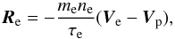
The inertial terms on the l.h.s. of Eq. (3) give a small contribution to the force balance
because of a small mass of both electrons and positrons. Gravitational force can also be
neglected because of the same reason. A gas pressure is much smaller than the magnetic
pressure in the force-free pulsar magnetosphere. Therefore, the momentum Eq. (3) reads in
the electron-positron plasma 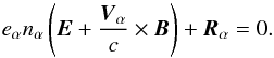 (4)Generally, the
friction force, Rα
contains two terms: one proportional to the difference of partial velocities (Ve − Vp)
and another proportional to the temperature gradient (see, e.g. Braginskii 1965). We will neglect the thermal contribution to
Rα and
take into account only friction caused by a difference in the partial velocities. This is
equivalent to neglecting the thermal diffusion of particles compared to their hydrodynamic
velocities. The friction force is related to the velocity difference, (Ve − Vp),
by a tensor that generally has components along and across the magnetic field and the
so-called Hall component, which is perpendicular to the both magnetic field and velocity
difference. In a strong magnetic field, parallel and perpendicular components are comparable
but the Hall component is small (see Braginskii 1965).
Therefore, we mimic the friction force between electrons and positrons by
(4)Generally, the
friction force, Rα
contains two terms: one proportional to the difference of partial velocities (Ve − Vp)
and another proportional to the temperature gradient (see, e.g. Braginskii 1965). We will neglect the thermal contribution to
Rα and
take into account only friction caused by a difference in the partial velocities. This is
equivalent to neglecting the thermal diffusion of particles compared to their hydrodynamic
velocities. The friction force is related to the velocity difference, (Ve − Vp),
by a tensor that generally has components along and across the magnetic field and the
so-called Hall component, which is perpendicular to the both magnetic field and velocity
difference. In a strong magnetic field, parallel and perpendicular components are comparable
but the Hall component is small (see Braginskii 1965).
Therefore, we mimic the friction force between electrons and positrons by
 (5)where τe is the
relaxation time of electrons. Note that this simple model for the friction force is often
used even for a magnetized plasma in laboratory conditions (Braginskii 1965) and yields qualitatively correct results. We assume that accuracy of
Eq. (5) is sufficient to study the magnetosphere of pulsars.
(5)where τe is the
relaxation time of electrons. Note that this simple model for the friction force is often
used even for a magnetized plasma in laboratory conditions (Braginskii 1965) and yields qualitatively correct results. We assume that accuracy of
Eq. (5) is sufficient to study the magnetosphere of pulsars.
It is usually more convenient to use linear combinations of Eq. (4) than to solve partial
equations. The sum of electron and positron Eq. (4) yields the equation of hydrostatic
equilibrium in the magnetosphere 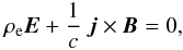 (6)where
ρe = e(np − ne) = eδn
is the charge density. Taking the difference between electron and positron Eq. (4), we
obtain the Ohm’s law in the form
(6)where
ρe = e(np − ne) = eδn
is the charge density. Taking the difference between electron and positron Eq. (4), we
obtain the Ohm’s law in the form 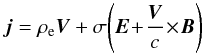 (7)where
σ = e2npτe/me
is the conductivity of plasma.
(7)where
σ = e2npτe/me
is the conductivity of plasma.
It was shown by Urpin (2012) that Eqs. (6), (7) are
equivalent to two equations 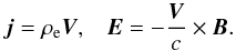 (8)These equations imply
that the force-free condition and the Ohm’s law (Eqs. (6), (7)) are equivalent to the
conditions of a frozen-in magnetic field and the presence of only advective currents in the
magnetosphere. Departures from this equivalence can be caused, for instance, by general
relativistic corrections (see Palenzuela 2013) but
they are very small in the magnetosphere. Note that the cross-production of the frozen-in
condition and B yields the well-known expression for the
transverse to B component of the velocity:
V⊥ = c(E × B/B2).
Certainly, the electric current should be non-vanishing in the magnetosphere,
j ≠ 0, because it maintains the magnetic
configuration. Hence, the hydrodynamic velocity should be non-zero as well since the current
is advective. Therefore, the force-free magnetosphere can only exist if hydrodynamic motions
are non-vanishing (Urpin 2012).
(8)These equations imply
that the force-free condition and the Ohm’s law (Eqs. (6), (7)) are equivalent to the
conditions of a frozen-in magnetic field and the presence of only advective currents in the
magnetosphere. Departures from this equivalence can be caused, for instance, by general
relativistic corrections (see Palenzuela 2013) but
they are very small in the magnetosphere. Note that the cross-production of the frozen-in
condition and B yields the well-known expression for the
transverse to B component of the velocity:
V⊥ = c(E × B/B2).
Certainly, the electric current should be non-vanishing in the magnetosphere,
j ≠ 0, because it maintains the magnetic
configuration. Hence, the hydrodynamic velocity should be non-zero as well since the current
is advective. Therefore, the force-free magnetosphere can only exist if hydrodynamic motions
are non-vanishing (Urpin 2012).
3. Equation governing the magnetospheric waves
Equation (8) should be complemented by the Maxwell equations. Then, the set of equations,
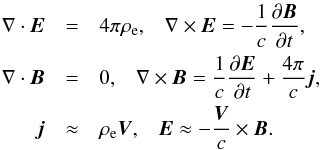
governing MHD processes in the force-free pulsar magnetosphere reads
 (9)Consider
the properties of MHD waves with small amplitudes as descibed by these equations. We assune
that the electric and magnetic fields are equal to E0
and B0 in the unperturbed
magnetosphere. The corresponding electric current, charge density, and velocity are
j0, ρe0. and
V0, respectively. For the sake
of simplicity, we assume that motions in the magnetosphere are non-relativistic
(V0 ≪ c). Linearising Eq.
(9), we obtain the set of equations that describes the behaviour of modes with a small
amplitude. Small perturbations are indicated by subscript 1. We consider waves with a short
wavelength. The space-time dependence of such waves can be taken in the form ∝exp(iωt − ik·r),
where ω and
k are the frequency and wave vector,
respectively. Such waves exist if their wavelength λ = 2π/k
is short compared to the characteristic length scale of the magnetosphere, L. Typically, L is greater than the stellar
radius. We search in MHD modes with the frequency to satisfy the condition ω < 1/τe,
since we use the MHD approach.
(9)Consider
the properties of MHD waves with small amplitudes as descibed by these equations. We assune
that the electric and magnetic fields are equal to E0
and B0 in the unperturbed
magnetosphere. The corresponding electric current, charge density, and velocity are
j0, ρe0. and
V0, respectively. For the sake
of simplicity, we assume that motions in the magnetosphere are non-relativistic
(V0 ≪ c). Linearising Eq.
(9), we obtain the set of equations that describes the behaviour of modes with a small
amplitude. Small perturbations are indicated by subscript 1. We consider waves with a short
wavelength. The space-time dependence of such waves can be taken in the form ∝exp(iωt − ik·r),
where ω and
k are the frequency and wave vector,
respectively. Such waves exist if their wavelength λ = 2π/k
is short compared to the characteristic length scale of the magnetosphere, L. Typically, L is greater than the stellar
radius. We search in MHD modes with the frequency to satisfy the condition ω < 1/τe,
since we use the MHD approach.
Substituting the frozen-in condition, E = −V × B/c,
into the equation c∇ × E = −∂B/∂t
and linearising the obtained induction equation, we have
 (10)A destabilising effect of
shear already has been studied by Urpin (2012). In the present paper, we concentrate on the
instability caused by the presence of electric currents in the magnetosphere. Therefore, we
assume that shear is small and neglect terms proportional to | ∂V0i/∂xj |.
Then, Eq. (10) reads
(10)A destabilising effect of
shear already has been studied by Urpin (2012). In the present paper, we concentrate on the
instability caused by the presence of electric currents in the magnetosphere. Therefore, we
assume that shear is small and neglect terms proportional to | ∂V0i/∂xj |.
Then, Eq. (10) reads  (11)where
 . The last term on
the r.h.s. is usually small compared to the third term (~λ/L) in a short
wavelength approximation. However, it becomes crucially important if the wavevector of
perturbations is almost perpendicular to B0.
. The last term on
the r.h.s. is usually small compared to the third term (~λ/L) in a short
wavelength approximation. However, it becomes crucially important if the wavevector of
perturbations is almost perpendicular to B0.
Substituting the expression j = ρeV
into Ampere’s law (second line of Eq. (9)) and linearising the obtained equation, we have
 (12)We search in relatively
low-frequency MHD modes with the frequency ω < ck. Note
that the frequency of MHD modes must satisfy the condition ω < 1/τe
because of the MHD approach used. The relaxation time can be estimated as τe ~ ℓe/ce,
where ce and ℓe are the thermal
velocity and mean free path of particles, respectively. The frequency ck can be greater or smaller
than 1/τe depending on a
wavelength λ.
If λ > 2πℓe(c/ce),
then we have ck < 1/τe.
If λ < 2πℓe(c/ce),
then we have ck > 1/τe.
(12)We search in relatively
low-frequency MHD modes with the frequency ω < ck. Note
that the frequency of MHD modes must satisfy the condition ω < 1/τe
because of the MHD approach used. The relaxation time can be estimated as τe ~ ℓe/ce,
where ce and ℓe are the thermal
velocity and mean free path of particles, respectively. The frequency ck can be greater or smaller
than 1/τe depending on a
wavelength λ.
If λ > 2πℓe(c/ce),
then we have ck < 1/τe.
If λ < 2πℓe(c/ce),
then we have ck > 1/τe.
By eliminating E1 from Eq. (12) by making
use of the linearised frozen-in condition and neglecting terms of the order of
(ω/ck)(V0/c),
we obtain the following for such modes:
 (13)The perturbation of the
charge density can be calculated from the equation ρe1 = ∇·E1/4π.
We have then with accuracy in terms of the lowest order in (λ/L)
(13)The perturbation of the
charge density can be calculated from the equation ρe1 = ∇·E1/4π.
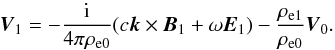
We have then with accuracy in terms of the lowest order in (λ/L)![Mathematical equation: \begin{equation} \rho_{\rm e1} \!=\! \frac{1}{4 \pi c} \left[ {\rm i} \vec{B}_0 \cdot (\vec{k} \!\times\! \vec{V}_1 \!) - {\rm i} \vec{V}_0 \cdot (\vec{k} \!\times\! \vec{B}_1 \!)\right]. \end{equation}](/articles/aa/full_html/2014/03/aa22105-13/aa22105-13-eq74.png) (14)Substituting Eq. (14)
into Eq. (13) and neglecting terms of the order of
(14)Substituting Eq. (14)
into Eq. (13) and neglecting terms of the order of  , we obtain the
second equation, which couples B1 and V1,
, we obtain the
second equation, which couples B1 and V1,
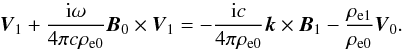
![Mathematical equation: \begin{eqnarray} 4 \pi c \rho_{\rm e0} \vec{V}_1 \! + \! {\rm i} \omega \vec{B}_0 \! \times \! \vec{V}_1 = -\, {\rm i} c^2 \vec{k} \! \times \! \vec{B}_1 \!-\! {\rm i} \vec{V}_0 \left[ \vec{B}_0 \! \cdot \! ( \vec{k} \! \times \! \vec{V}_1 \! )\right]. \end{eqnarray}](/articles/aa/full_html/2014/03/aa22105-13/aa22105-13-eq78.png) (15)Eliminating
B1 from Eqs. (11) and (15) in
favor of V1 and again neglecting terms
of the order of (ω/ck)(V0/c)
and (ω/ck)2,
we obtain the equation for V1 in the form
(15)Eliminating
B1 from Eqs. (11) and (15) in
favor of V1 and again neglecting terms
of the order of (ω/ck)(V0/c)
and (ω/ck)2,
we obtain the equation for V1 in the form
![Mathematical equation: \begin{equation} 4 \pi \! c \rho_{\rm e0} \! \vec{V}_{1} - {\rm i} \frac{c^2}{\tilde{\omega}} (\vec{k} \! \cdot \! \vec{B}_0) \vec{k} \! \times \!\!\vec{V}_{1} \!\!=\! \frac{c^2}{\tilde{\omega}} \vec{k} \! \times \! [ (\!\vec{V}_{1} \!\! \cdot \!\! \nabla \!) \vec{B}_0 \!-\!{\rm i} \vec{B}_0 (\vec{k} \! \cdot \!\! \vec{V}_{1}) ]. \end{equation}](/articles/aa/full_html/2014/03/aa22105-13/aa22105-13-eq81.png) (16)It immediately follows from
this equation that (k·V1) = 0
and, hence, the magnetospheric waves are transverse. Equation (16) is simplified to
(16)It immediately follows from
this equation that (k·V1) = 0
and, hence, the magnetospheric waves are transverse. Equation (16) is simplified to
 (17)where
 (18)In
the case of a uniform magnetic field, Eq. (17) reduces to the equation considered by Urpin
(2011).
(18)In
the case of a uniform magnetic field, Eq. (17) reduces to the equation considered by Urpin
(2011).
4. Dispersion equation and instability of magnetospheric modes
Generally, the stability properties of perturbations are complicated even in the local
approximation. Equation (17) can be transformed to a more convenient form that does not
contain a cross production of k and V1.
Calculating the cross production of k and Eq. (17) and taking into account
k·V1 = 0,
we have ![Mathematical equation: \begin{equation} \vec{k} \times \vec{V}_1 = - \frac{1}{\alpha} \left\{ {\rm i} k^2 (\vec{k} \cdot \vec{B}_0) \vec{V}_1 - (\vec{V}_1 \cdot \nabla) [ \vec{k} \times (\vec{k}\times \vec{B}_0)] \right\}. \end{equation}](/articles/aa/full_html/2014/03/aa22105-13/aa22105-13-eq87.png) (19)Substituting this
expression into Eq. (17), we obtain
(19)Substituting this
expression into Eq. (17), we obtain ![Mathematical equation: \begin{eqnarray} \left[ \alpha^2 - k^2 (\vec{k} \cdot \vec{B}_0)^2 \right] \vec{V}_1 = \alpha (\vec{V}_1 \cdot \nabla) \vec{k} \times \vec{B}_0 \nonumber \\ + \,{\rm i}(\vec{k} \cdot \vec{B}_0) (\vec{V}_1 \cdot \nabla) [ \vec{k} (\vec{k} \cdot \vec{B}_0) - k^2 \vec{B}_0 ]. \end{eqnarray}](/articles/aa/full_html/2014/03/aa22105-13/aa22105-13-eq88.png) (20)The
magnetospheric waves can exist in the force-free pulsar magnetosphere only if the wavevector
k and the unperturbed magnetic field
B0 are almost (but not exactly)
perpendicular and the scalar production (k·B0)
is small but non-vanishing (see Urpin 2011, 2012). The reason for this is clear from simple
qualitative arguments. The magnetospheric waves are transverse (k·V1 = 0),
and the velocity of plasma is perpendicular to the wave vector. However, wave motions across
the magnetic field in a strong field are suppressed and the velocity component along the
magnetic field should be much greater than in the transverse (see, e.g. Mestel &
Shibata 1994). Therefore, the direction of a
wavevector k should be close to the plane
perpendicular to B0. That is why we treat Eq.
(20) only in the case of small (k·B0).
(20)The
magnetospheric waves can exist in the force-free pulsar magnetosphere only if the wavevector
k and the unperturbed magnetic field
B0 are almost (but not exactly)
perpendicular and the scalar production (k·B0)
is small but non-vanishing (see Urpin 2011, 2012). The reason for this is clear from simple
qualitative arguments. The magnetospheric waves are transverse (k·V1 = 0),
and the velocity of plasma is perpendicular to the wave vector. However, wave motions across
the magnetic field in a strong field are suppressed and the velocity component along the
magnetic field should be much greater than in the transverse (see, e.g. Mestel &
Shibata 1994). Therefore, the direction of a
wavevector k should be close to the plane
perpendicular to B0. That is why we treat Eq.
(20) only in the case of small (k·B0).
Consider Eq. (20) in the neighbourhood of a point, r0,
using local Cartesian coordinates. We assume that the z-axis is parallel to the
local direction of the unperturbed magnetic field and the corresponding unit vector is
b = B0(r0)/B0(r0).
The wavevector can be represented as k = k∥b + k⊥,
where k∥ and k⊥
are parallel and perpendicular to the magnetic field components of k, respectively.
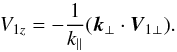
Then, we have from the continuity equation
 (21)Since k⊥ ≫ k∥, we have
V1z ≫ V1 ⊥
and, hence, (V1·∇) ≈ V1z∂/∂z.
Therefore, the z-component of Eq. (20) yields the following dispersion
relation
(21)Since k⊥ ≫ k∥, we have
V1z ≫ V1 ⊥
and, hence, (V1·∇) ≈ V1z∂/∂z.
Therefore, the z-component of Eq. (20) yields the following dispersion
relation 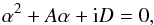 (22)where
![Mathematical equation: \begin{eqnarray} A&=& (\vec{k} \times \vec{b}) \cdot \frac{\partial \vec{B}_0}{\partial z}, \nonumber \\ D &=& k^2 (\vec{k} \cdot \vec{B}_0) \left[ \vec{b} \cdot \frac{\partial \vec{B}_0}{\partial z} + {\rm i} (\vec{k} \cdot \vec{B}_0) \right]. \end{eqnarray}](/articles/aa/full_html/2014/03/aa22105-13/aa22105-13-eq102.png) (23)We
neglect in D
corrections of the order ~λ/L to
k2(k·B0)2.
The roots of Eq. (22) correspond to two modes with the frequencies given by
(23)We
neglect in D
corrections of the order ~λ/L to
k2(k·B0)2.
The roots of Eq. (22) correspond to two modes with the frequencies given by
 (24)If the magnetic field
is approximtely uniform along the field lines, then ∂B0/∂z ≈ 0,
and, hence, A ≈ 0 and D ≈ ik2(k·B0)2.
In this case, the magnetospheric modes are stable and
(24)If the magnetic field
is approximtely uniform along the field lines, then ∂B0/∂z ≈ 0,
and, hence, A ≈ 0 and D ≈ ik2(k·B0)2.
In this case, the magnetospheric modes are stable and
 .
The corresponding frequency is
.
The corresponding frequency is 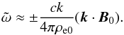 (25)These waves have been
first studied by Urpin (2011). Deriving the
dispersion Eq. (25), it was assumed that ω ≪ ck. Therefore, the
magnetospheric waves can exist only if (k·B0)
is small, as was discussed above: (k·B0) ≪ 4πρe0.
Sometimes, it is convenient to measure the true charge density, ρe0, in units of
the Goldreich-Julian charge density, ρGJ = ΩB0/2πc,
where Ω is the angular velocity
of a pulsar. Then, we can suppose ρe0 = ξρGJ,
where ξ is a
dimensionless parameter and, hence, the condition ω ≪ ck transforms into
(25)These waves have been
first studied by Urpin (2011). Deriving the
dispersion Eq. (25), it was assumed that ω ≪ ck. Therefore, the
magnetospheric waves can exist only if (k·B0)
is small, as was discussed above: (k·B0) ≪ 4πρe0.
Sometimes, it is convenient to measure the true charge density, ρe0, in units of
the Goldreich-Julian charge density, ρGJ = ΩB0/2πc,
where Ω is the angular velocity
of a pulsar. Then, we can suppose ρe0 = ξρGJ,
where ξ is a
dimensionless parameter and, hence, the condition ω ≪ ck transforms into
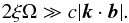 (26)Obviously, this condition
can be satisfied only for waves with the wavevector almost perpendicular to B0.
Note, however, that if k is exactly perpendicular to
B0 the magnetospheric waves do
not exist.
(26)Obviously, this condition
can be satisfied only for waves with the wavevector almost perpendicular to B0.
Note, however, that if k is exactly perpendicular to
B0 the magnetospheric waves do
not exist.
If ∂B0/∂z ≠ 0,
the magnetospheric waves turn out to be unstable. The instability is especially pronounced
if | k·B0 | < B0/L.
In this case, the second term in the brackets of Eq. (24) is smaller than the first one and,
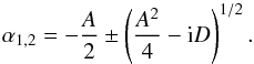
therefore, the roots are 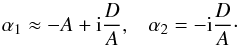 (27)The coefficient
D is
approximately equal to
(27)The coefficient
D is
approximately equal to 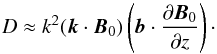 (28)The first and second roots
of Eq. (27) correspond to oscillatory and non-oscillatory modes, respectively. The occurence
of instability is determined by the sign of the ratio D/A. If this ratio is positive
for some wavevector k, then the non-oscillatory mode is
unstable but the oscillatory one is stable for such k. If
D/A < 0, then the oscillatory
mode is unstable but the non-oscillatory one is stable for corresponding k. Note,
however, that the frequency of oscillatory modes often can be very high and ω ≫ ck. Our
consideration does not apply in this case. Indeed, we have α1 ~ A and, hence,
(28)The first and second roots
of Eq. (27) correspond to oscillatory and non-oscillatory modes, respectively. The occurence
of instability is determined by the sign of the ratio D/A. If this ratio is positive
for some wavevector k, then the non-oscillatory mode is
unstable but the oscillatory one is stable for such k. If
D/A < 0, then the oscillatory
mode is unstable but the non-oscillatory one is stable for corresponding k. Note,
however, that the frequency of oscillatory modes often can be very high and ω ≫ ck. Our
consideration does not apply in this case. Indeed, we have α1 ~ A and, hence,
 . The condition ω ≪ ck
implies that B0/4πρe0L < 1.
Expressing the charge density in units of the Goldreich-Julian density, ρe0 = ξρGJ,
we transform this inequality into
. The condition ω ≪ ck
implies that B0/4πρe0L < 1.
Expressing the charge density in units of the Goldreich-Julian density, ρe0 = ξρGJ,
we transform this inequality into 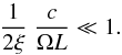 (29)This condition can be
satisfied only in regions where ξ ≫ 1 and the charge density is much greater than the
Goldreich-Julian density. If inequality (29) is not fulfilled, then Eq. (27) for the
oscillatory mode α1 does not apply, and only the
non-oscillatory modes exist. For example, the charge density is large in the region where
the electron-positron plasma is created. Therefore, condition (29) can be satisfied there,
and, hence, the oscillatory instability can occur in this region.
(29)This condition can be
satisfied only in regions where ξ ≫ 1 and the charge density is much greater than the
Goldreich-Julian density. If inequality (29) is not fulfilled, then Eq. (27) for the
oscillatory mode α1 does not apply, and only the
non-oscillatory modes exist. For example, the charge density is large in the region where
the electron-positron plasma is created. Therefore, condition (29) can be satisfied there,
and, hence, the oscillatory instability can occur in this region.
The non-oscillatory modes have a lower growth rate and usually can occur in the pulsar magnetosphere. For any magnetic configuration, it is easy to verify that one can choose the wavevector of perturbations, k, in such a way that the ratio D/A becomes positive, and, hence, the non-oscillatory mode is unstable. Indeed, we can represent k as the sum of components parallel and perpendicular to the magnetic field, k = k∥ + k⊥. Obviously, A ∝ k⊥ and D ∝ k∥ and, hence, A/D ∝ k∥/k⊥. Therefore, if A/D < 0 for a value of k = (k∥,k⊥), this ratio changes the sign for k = (−k∥,k⊥) and k = (k∥, −k⊥), and waves with such the wavevectors are unstable. It turns out that there always exists the range of wavevectors for which the non-oscillatory modes are unstable and, hence, the force-free magnetosphere is always the subject of instability.
The necessary condition of instability is D ≠ 0. As it was mentioned, the magnetospheric waves
exist only if the wavevector k is close to the plane perpendicular
to the unperturbed magnetic field, B0, and the scalar
production (k·B0)
is small (but non-vanishing). Therefore, the necessary condition D ≠ 0 is equivalent to
b·(∂B0/∂z) ≠ 0.
Since b = B0/B0,
we can rewrite this condition as 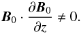 (30)This condition is
satisfied if the magnetic pressure gradient along the magnetic field is non-zero. The
topology of the magnetic field can be fairly complicated in the magnetosphere, particularly
in a region close to the neutron star. This may happen because the field geometry at the
neutron star surface should be very complex (see, e.g. Bonanno et al. 2005, 2006). Therefore, Eq. (30) can be satisfied in different regions of
the magnetosphere. However, this condition can be fulfilled even if the magnetic
configuration is relatively simple. As a possible example, we consider a region near the
magnetic pole of a neutron star. It was shown by Urpin (2012) that a special type of cylindrical waves can exist there with
m ≠ 0, where
m is the
azimuthal wavenumber. The criterion of instability (30) is certainly satisfied in this
region and, hence, the instability can occur. Indeed, one can mimic the magnetic field by a
vacuum dipole near the axis. The radial and polar components of the dipole field in the
spherical coordinates (r,θ,ϕ) are
(30)This condition is
satisfied if the magnetic pressure gradient along the magnetic field is non-zero. The
topology of the magnetic field can be fairly complicated in the magnetosphere, particularly
in a region close to the neutron star. This may happen because the field geometry at the
neutron star surface should be very complex (see, e.g. Bonanno et al. 2005, 2006). Therefore, Eq. (30) can be satisfied in different regions of
the magnetosphere. However, this condition can be fulfilled even if the magnetic
configuration is relatively simple. As a possible example, we consider a region near the
magnetic pole of a neutron star. It was shown by Urpin (2012) that a special type of cylindrical waves can exist there with
m ≠ 0, where
m is the
azimuthal wavenumber. The criterion of instability (30) is certainly satisfied in this
region and, hence, the instability can occur. Indeed, one can mimic the magnetic field by a
vacuum dipole near the axis. The radial and polar components of the dipole field in the
spherical coordinates (r,θ,ϕ) are
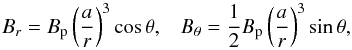 (31)where Bp is the polar
strength of the magnetic field at the neutron star surface and a is the stellar radius (see,
e.g. Urpin et al. 1994). The radial field is much
greater than the polar one near the axis and, therefore, it is easy to check that the
criterion of instability (30) is fulfilled in the polar gap. Hence, filament-like structures
can be formed there. In some models, note that the force-free field at the top of the polar
gap can differ from that of a vacuum dipole (see, e.g. Petrova 2012) but this cannot change our conclusion qualitatively. We will
consider the instability in the polar gap in more detail elsewhere.
(31)where Bp is the polar
strength of the magnetic field at the neutron star surface and a is the stellar radius (see,
e.g. Urpin et al. 1994). The radial field is much
greater than the polar one near the axis and, therefore, it is easy to check that the
criterion of instability (30) is fulfilled in the polar gap. Hence, filament-like structures
can be formed there. In some models, note that the force-free field at the top of the polar
gap can differ from that of a vacuum dipole (see, e.g. Petrova 2012) but this cannot change our conclusion qualitatively. We will
consider the instability in the polar gap in more detail elsewhere.
From Eq. (30), it follows that the instability in pulsar magnetospheres is driven by a non-uniformity of the magnetic pressure and, hence, it can be called “the magnetic pressure-driven instability”. Note that this instability can occur only in plasma with a non-zero charge density, ρe0 ≠ 0, and does not arise in a neutral plasma with ρe0 = 0.
5. Discussion
We have considered stability of the electron-positron plasma in the magnetosphere of
pulsars. The pair plasma in the magnetosphere is likely created in a two-stage process:
primary particles are accelerated by an electric field parallel to the magnetic field near
the poles up to extremely high energy, and these produce a secondary, denser pair plasma via
a cascade process (see, e.g. Michel 1982). The number
density of this secondary plasma greatly exceeds the Goldreich-Julian number density,
nGJ = | ρGJ | /e,
required to maintain a corotation electric field and, hence, the multiplicity factor
ξ can be very
large. Unfortunately, this factor is model dependent and rather uncertain with estimates in
a wide range from 102
to 106 (see, e.g.
Gedalin et al. 1998). For example, the model of
bound-pair creation above polar caps (Usov & Melrose 1996) results in a relatively
low value of ξ.
This model postulates that the photons emitted by primary particles as a result of curvature
emission create bound pairs (positronium) rather than free pairs. While the pairs remain
bound, the screening of the component E parallel to the magnetic field is
inefficient because screening is attributed to free pairs that can be charge-separated as a
result of acceleration by E∥. In the absence of
screening, the height of the polar gap and the maximum energy of primary particles increase.
The main part of the energy that primary particles gain during their motion through the
polar gap is transformed into the energy of curvature photons and then into the energy of
secondary pairs. Assuming that the electric field in the gap has more or less standard value
(~1010 V cm-1), Usov & Melrose (1996)
obtain the following estimate for the multiplicity factor above polar caps:
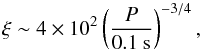 (32)where P is the pulsar period. Note
that this value can be higher if dissociation of bound pairs is taken into account. However,
the instability can operate in the region of pair creation even if ξ is such small. It can be
efficient in regions with ξ ~ 1 as well.
(32)where P is the pulsar period. Note
that this value can be higher if dissociation of bound pairs is taken into account. However,
the instability can operate in the region of pair creation even if ξ is such small. It can be
efficient in regions with ξ ~ 1 as well.
The geometry of motions in the unstable magnetospheric waves is simple. Since these waves are transverse (k·V1 = 0) and the wavevector of such waves should be close to the plane perpendicular to B0, plasma motions are almost parallel or anti-parallel to the magnetic field. The velocity across B0 is small. In our model, we have only considered the stability of plane waves using a local approximation. In this model, the instability should lead to formation of filament-like structures with filaments alongside the magnetic field lines. Note that plasma can move in the opposite directions in different filaments. The characteristic timescale of formation of such structures is ~1/Imω. Since the necessary condition (30) is likely satisfied in a major fraction of a magnetosphere, one can expect that filament-like structures can appear (and disappear) in different magnetospheric regions. We used the hydrodynamic approach in our consideration, which certainly does not apply to a large distance from the pulsar where the number density of plasma is small. Therefore, the considered instability is most likely efficient in the inner part of a magnetosphere where filament-like structures can be especially pronounced. The example of a region where the instability can occur is the so-called dead zone. Most likely, the hydrodynamic approximation is valid in this region and hydrodynamic motions are non-relativistic, as it was assumed in our analysis. Note that a particular geometry of motions in the basic (unperturbed) state is not crucial for the instability and cannot suppress the formation of filament-like structures. These structures can be responsible for fluctuations of plasma and, hence, the magnetospheric emission can fluctuate with the same characteristic timescale.
It should be also noted that the considered instability is basically electromagnetic in origin as followed in our treatment. Hydrodynamic motions in the basic state play no important role in the instability. For instance, the unperturbed velocity does even not enter the expression for the growth rate. Therefore, one can expect that the same type of instability arises in the regions where velocities are relativistic. This case will be considered in detail elsewhere.
Hydrodynamic motions accompanying the instability can be the reason of turbulent diffusion in the magnetosphere. This diffusion should be highly anisotropic because both the criteria of instability and its growth rate are sensitive to the direction of the wave vector. However, the turbulent diffusion caused by motions may be efficient in the transport of angular momentum and mixing plasma with a much higher enhancement of the diffusion coefficient in the direction of the magnetic field since the velocity of motions across the field is much slower than along it.
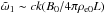
The characteristic growth rate of unstable waves, Im ω, can be estimated from Eq.
(27) as Im ω ~ (c/4πρe0)(D/A).
Since k and B0
should be close to orthogonality in magnetospheric waves, we have A ~ kB0/L
and  , where we
estimate b·(∂B0/∂z)
as B0/L.
Then,
, where we
estimate b·(∂B0/∂z)
as B0/L.
Then, 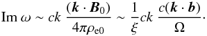 (33)Like stable
magnetospheric modes, the unstable ones can occur in the magnetosphere if Eq. (26) is
satisfied. Generally, this condition requires a position close to orthogonality of (but not
orthogonal) k and B0.
Under certain conditions, however, the instability can arise even if departures from
orthogonality are not very small but ξ ≫ 1. As it was mentioned, this can happen in
regions where the electron-positron plasma is created. The parameter ξ can also be greater than 1
in those regions where plasma moves with the velocity greater ΩL. Indeed, we have
ρe0 = (1/4π)∇·E0
for the unperturbed charge density. Since E0 is determined by the
frozen-in condition (8), we obtain ρe0 ~ (1/4πcL)V0B0.
If the velocity of plasma in a magnetosphere is greater than the rotation velocity, then
ξ ~ V0/ΩL.
Some models predict that the velocity in the magnetisphere can reach a fraction of
c. Obviously,
in such regions, condition (26) is satisfied even if departures from orthogonality of
k and B0
are relatively large.
(33)Like stable
magnetospheric modes, the unstable ones can occur in the magnetosphere if Eq. (26) is
satisfied. Generally, this condition requires a position close to orthogonality of (but not
orthogonal) k and B0.
Under certain conditions, however, the instability can arise even if departures from
orthogonality are not very small but ξ ≫ 1. As it was mentioned, this can happen in
regions where the electron-positron plasma is created. The parameter ξ can also be greater than 1
in those regions where plasma moves with the velocity greater ΩL. Indeed, we have
ρe0 = (1/4π)∇·E0
for the unperturbed charge density. Since E0 is determined by the
frozen-in condition (8), we obtain ρe0 ~ (1/4πcL)V0B0.
If the velocity of plasma in a magnetosphere is greater than the rotation velocity, then
ξ ~ V0/ΩL.
Some models predict that the velocity in the magnetisphere can reach a fraction of
c. Obviously,
in such regions, condition (26) is satisfied even if departures from orthogonality of
k and B0
are relatively large.
The growth rate of instability (31) is sufficiently high and can reach a fraction of ck. For example, if a pulsar rotates with the period 0.01 s and ξ ~ 1, magnetospheric waves with the wavelength ~105−106 cm grow on a timescale ~10-4−10-5 s if a departure from orthogonality between k and B0 is of the order of 10-4. The considered instability can occur everywhere in the magnetosphere except regions close to the surfaces where B0·(∂B0/∂z) = 0 and instability criterion (30) is not satisfied.
The instability considered is caused by a combined action of non-uniform magnetic field and non-zero charge density. Certainly, this is not the only instability that can occur in the pulsar magnetosphere. There are many factors that can destabilize a highly magnetized magnetospheric plasma and lead to various instabilities with substantially different properties. For instance, differential rotation predicted by many models of the magnetosphere can be the reason of instability as was shown by Urpin (2012). This instability is closely related to the magnetorotational instability (Velikhov 1959) which is well-studied in the context of accretion disks (see, e.g. Balbus & Hawley 1991). Generally, the regions, where rotation is differential and the magnetic field is non-unifom, can overlap. Thus, the criteria of both instabilities can be fulfilled in the same region. However, these instabilities usually have substantially different growth rates. The instability caused by differential rotation arises usually on a time-scale comparable to the rotation period of a pulsar. The growth rate of the magnetic pressure-driven instability is given by Eq. (30) and can even reach a fraction of ck in accordance with our results. Therefore, this instability occurs
typically on a shorter time-scale than the instability caused by differential rotation. If two different instabilities can occur in the same region, then, the instability with a shorter growth time usually turns out to be more efficient and determines plasma fluctuations. It is likely, therefore, that the magnetic pressure-driven instability is more efficient everywhere in the magnetosphere except surfaces where criterion (30) is not satisfied. In the neighbourhood of these surfaces, howevere, the instability associated with differential rotation can occur despite it arises on a longer time-scale. Therefore, it appears that the whole pulsar magnetosphere should be unstable.
Instabilities can lead to a short-term variability of plasma and, hence, to modulate the magnetospheric emission of pulsars. The unstable plasma can also modulate the radiation produced at the stellar surface and propagating through the magnetosphere. Since the growth time of magnetospheric waves can be substantially different in different regions, the instability can lead to a generation of fluctuations over a wide range of timescales, including those yet to be detected in the present and future pulsar searches (Liu et al. 2011; Stappers et al. 2011). Detection of such fluctuations would uncover the physical conditions in the magnetosphere and enable one to construct a relevant model of the pulsar magnetosphere and its observational manifestations beyond the framework of the classical concept (see, e.g. Kaspi 2010).
Acknowledgments
The author thanks the Russian Academy of Sciencs for financial support under the programme OFN-15.
References
- Balbus, S., & Hawley, J. 1991, ApJ, 376, 214 [NASA ADS] [CrossRef] [Google Scholar]
- Beskin, V. 1997, Uspekhi Fizicheskikh Nauk, 167, 689 [CrossRef] [Google Scholar]
- Bonanno, A., & Urpin, V. 2008a, A&A, 477, 35 [NASA ADS] [CrossRef] [EDP Sciences] [Google Scholar]
- Bonanno, A., & Urpin, V. 2008b, A&A, 488, 1 [NASA ADS] [CrossRef] [EDP Sciences] [Google Scholar]
- Bonanno, A., Urpin, V, & Belvedere, G. 2005, A&A, 440, 199 [NASA ADS] [CrossRef] [EDP Sciences] [Google Scholar]
- Bonanno, A., Urpin, V, & Belvedere, G. 2006, A&A, 451, 1049 [NASA ADS] [CrossRef] [EDP Sciences] [Google Scholar]
- Braginskii, S. 1965, Rev. Plasma Phys., 1, 205 [NASA ADS] [Google Scholar]
- Contopoulos, I., Kazanas, D., & Fendt, C. 1999, ApJ, 511, 351 [Google Scholar]
- Davidson, R. 1990, Physics of non-neutral plasmas (Addison-Wesley Publishing Company) [Google Scholar]
- Davidson, R., & Felice, G. 1998, Phys. Plasma, 5, 3497 [NASA ADS] [CrossRef] [Google Scholar]
- Fung, P. K., Khechinashvili, D., & Kuijpers, J. 2006, A&A, 445, 779 [NASA ADS] [CrossRef] [EDP Sciences] [Google Scholar]
- Gedalin, M., Melrose, D., & Gruman, E. 1998, Phys. Rev. E, 57, 3399 [NASA ADS] [CrossRef] [Google Scholar]
- Goodwin, S., Mestel, J., Mestel, L., & Wright, G. 2004, MNRAS, 349, 213 [NASA ADS] [CrossRef] [Google Scholar]
- Kaspi, V. M. 2010, PNAS, 107, 7147 [Google Scholar]
- Komissarov, S. 2006, MNRAS, 367, 19 [NASA ADS] [CrossRef] [Google Scholar]
- Levy, R. 1965, Phys. Fluids, 8, 1288 [NASA ADS] [CrossRef] [MathSciNet] [Google Scholar]
- Liu, K., Verbiest, J. P. W., Kramer, M., et al. 2011, MNRAS, 417, 2916 [NASA ADS] [CrossRef] [Google Scholar]
- McKinney, J. C. 2006, MNRAS, 368, L30 [NASA ADS] [CrossRef] [Google Scholar]
- Mestel, L. 1973, Ap&SS, 24, 289 [NASA ADS] [CrossRef] [Google Scholar]
- Mestel, L., & Shibata, S. 1994, MNRAS, 271, 621 [NASA ADS] [Google Scholar]
- Michel, F. 1973, ApJ, 180, L133 [NASA ADS] [CrossRef] [Google Scholar]
- Michel, F. 1982, Rev. Mod. Phys., 54, 1 [NASA ADS] [CrossRef] [Google Scholar]
- Palenzuela, C. 2013, MNRAS, 431, 1852 [CrossRef] [Google Scholar]
- Petri, J., Heyvaerts, J., & Bonazzola, S. 2002, A&A, 287, 520 [NASA ADS] [CrossRef] [EDP Sciences] [Google Scholar]
- Petri, J., Heyvaerts, J., & Bonazzola, S. 2003, A&A, 411, 203 [NASA ADS] [CrossRef] [EDP Sciences] [Google Scholar]
- Petrova, S. 2012, MNRAS, 427, 514 [NASA ADS] [CrossRef] [Google Scholar]
- Petrova, S. 2013, ApJ, 764, 129 [NASA ADS] [CrossRef] [Google Scholar]
- Stappers, B. W., Hessels, J. W. T., Alexov, A., et al. 2011, A&A, 530, A80 [NASA ADS] [CrossRef] [EDP Sciences] [Google Scholar]
- Tayler, R. 1973a, MNRAS, 161, 365 [NASA ADS] [CrossRef] [Google Scholar]
- Tayler, R. 1973b, MNRAS, 163, 77 [NASA ADS] [CrossRef] [Google Scholar]
- Timokhin, A. 2006, MNRAS, 368, 1055 [Google Scholar]
- Urpin, V. 2011, A&A, 535, L5 [NASA ADS] [CrossRef] [EDP Sciences] [Google Scholar]
- Urpin, V. 2012, A&A, 541, A117 [NASA ADS] [CrossRef] [EDP Sciences] [Google Scholar]
- Urpin, V., Chanmugam, G., & Sang, Y. 1994, ApJ, 433, 780 [NASA ADS] [CrossRef] [Google Scholar]
- Velikhov, E. 1959, Sov. Phys. JETP, 9, 995 [Google Scholar]
Current usage metrics show cumulative count of Article Views (full-text article views including HTML views, PDF and ePub downloads, according to the available data) and Abstracts Views on Vision4Press platform.
Data correspond to usage on the plateform after 2015. The current usage metrics is available 48-96 hours after online publication and is updated daily on week days.
Initial download of the metrics may take a while.