| Issue |
A&A
Volume 562, February 2014
|
|
|---|---|---|
| Article Number | A85 | |
| Number of page(s) | 6 | |
| Section | Planets and planetary systems | |
| DOI | https://doi.org/10.1051/0004-6361/201322251 | |
| Published online | 11 February 2014 | |
Rotationally resolved spectroscopy of (20000) Varuna in the near-infrared
1
Fundación Galileo Galilei-INAF, Rambla José Ana Fernández Pérez 7, 38712
Breña Baja,
TF
Spain
e-mail:
This email address is being protected from spambots. You need JavaScript enabled to view it.
2
University of Tennessee, Knoxville
TN
37996,
USA
3
Instituto Astrofísico de Canarias, IAC, Spain
4
Carl Sagan Center, SETI Institute and NASA Ames Research Center,
CA,
USA
Received: 10 July 2013
Accepted: 9 December 2013
Abstract
Context. Models of the escape and retention of volatiles by minor icy objects exclude any presence of volatile ices on the surface of trans-Neptunian objects (TNOs) smaller than ~1000 km in diameter at the typical temperature in this region of the solar system, whereas the same models show that water ice is stable on the surface of objects over a wide range of diameters. Collisions and cometary activity have been used to explain the process of surface refreshing of TNOs and Centaurs. These processes can produce surface heterogeneity that can be studied by collecting information at different rotational phases.
Aims. The aims of this work are to study the surface composition of (20000) Varuna, a TNO with a diameter 668+154-86 km and to search for indications of rotational variability.
Methods. We observed (20000) Varuna during two consecutive nights in January 2011 with the near-infrared camera and spectrometer NICS at the Telescopio Nazionale Galileo, La Palma, Spain. We used the low resolution mode with the AMICI prism to obtain a set of spectra covering the whole rotation period of the Varuna (Pr = 6.34 h). We fit the resulting relative reflectance with radiative transfer models of the surface of atmosphereless bodies.
Results. After studying the spectra corresponding to different rotational phases of Varuna, we did not find any indication of surface variability at 2σ level. In all the spectra, we detect an absorption at 2.0 μm, suggesting the presence of water ice on the surface. We do not detect any other volatiles on the surface, although the signal-to-noise ratio is not high enough to discard their presence in small quantities. Based on scattering models, we present two possible compositions compatible with our set of data and discuss their implications in the framework of the collisional history of the trans-Neptunian belt.
Conclusions. We find that the most probable composition for the surface of Varuna is a mixture of amorphous silicates, complex organics, and water ice. This composition is compatible with all the materials being primordial, so no replenishment mechanism is needed in the equation. However, our data can also be fitted by models containing up to a 10% of methane ice. For an object with the characteristics of Varuna, this volatile could not be primordial, so an event, such as an energetic impact, would be needed to explain its presence on the surface.
Key words: Kuiper belt objects: individual: (2000) Varuna / methods: observational / methods: numerical / techniques: spectroscopic / planets and satellites: composition
© ESO, 2014
1. Introduction
Trans-Neptunian objects (TNOs) are thought to be composed mainly of the less processed material from the protosolar nebula. The study of their surface composition and their dynamical and physical properties provides important information for understanding the conditions of the early solar system environment. Investigation of visible and near-infrared (NIR) spectra of TNOs and Centaurs (a population of icy objects related to the TNOs and the Jupiter family comets) show a wide range of compositions. Some objects are covered by dark irradiation mantles showing a mostly featureless and neutral-to-reddish spectrum in the visible and NIR. Some other objects have retained large amounts of ices (e.g., CH4, N2, H2O) on their surfaces. The spectra of these objects are characterized by clear absorption bands that appear over the entire wavelength range from the visible to the NIR. However, most of the objects show intermediate surface compositions, i.e., a mixture of ices and irradiated mantles. Most of these objects are not able to retain volatiles, but water ice can be present on their surface.
Barucci et al. (2011) and Brown et al. (2012b) study the possibility of water ice on the surfaces of TNOs and Centaurs from extensive collections of spectra of these minor bodies. Both works agree on the broad results. Most of the objects brighter than an absolute magnitude of H = 3 have deep water ice absorption. For those fainter than an absolute magnitude of H = 5, deep water ice absorption is never seen. For the intermediate objects, those with a diameter ~650 km, only one (2003 AZ84) shows a deep water ice absorption band.
TNOs and Centaurs with a clear detection of water ice are found in all the taxonomic groups, except for the IR taxonomic group introduced in Barucci et al. (2008) (objects with a red intermediate slope). Moreover, they are found in all the dynamical classes, except the cold classical population (Barucci et al., 2011).
According to the Minor Planet Center (MPC), (20000) Varuna (hereafter Varuna) is a classical TNO (a,e,i = 43.189 AU,0.053,17.1°) with a magnitude H = 3.6. It has an estimated diameter of  km (Lellouch et al. 2013). Its surface composition has been studied through NIR spectroscopy by Licandro et al. (2001) and Barkume et al. (2008). These authors, however, reach different conclusions. Licandro et al. (2001) find a hint of an absorption of water ice around 2.0 μm on a reddish NIR spectrum, while Barkume et al. (2008) show a featureless spectrum with a blue slope in the H band. They interpret these contradictory results as indicating surface heterogeneity.
In this work, we present the results of a observational campaign designed to study the surface composition of Varuna at different rotational phases. The purpose of this work is to investigate the possibility of inhomogeneity suggested in previous studies.
2. Observations and data
In January 2011 we observed Varuna during two consecutive nights using the 3.58 m Telescopio Nazionale Galileo (TNG), situated at the “Roque de los Muchachos” observatory in La Palma, Canary Islands, Spain. We used the high-throughput low resolution mode of the Near-Infrared Camera and Spectrometer (NICS), with an Amici prism disperser and the 1′′ slit. This mode yields a 0.8−2.5 μm spectrum with a constant resolving power of R ≃ 50. The slit was oriented at the parallactic angle (and updated during the night), and the tracking of the telescope was set to compensate for the nonsideral motion of the TNO.
We observed the object each night during several hours, in order to entirely cover its rotation period Pr = 6.34 h (Thirouin et al., 2010). The series of spectra consisted of consecutive exposures of 90 s following an ABBA scheme, where A is the position of the object in the slit during the first acquisition and B a position shifted 10′′ along the slit. The ABBA scheme was repeated several times in order to increase the signal-to-noise ratio (S/N) and to cover the whole rotation period. To study possible spectral variations with the rotational phase, we divided the AB pairs into four groups, each covering a quarter of the rotation. Then we combined each AB pair to remove the sky contribution from the spectra. After discarding those spectra with low S/N (probably due to nonphotometric conditions), we kept 114 spectra for Phase 1, 36 for Phase 2, 48 for Phase 3, and 68 for Phase 4, for total exposure times of 10 260, 3240, 4320, and 6120 s, respectively (see Table 1). We combined all the spectra of each group, obtaining a spectrum for each phase that we extracted and calibrated using IRAF standard packages as described in Licandro et al. (2001).
Date and time (UT) of the observations and total exposure time corresponding to the four rotational phases in which we divided our Varuna data.
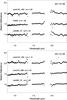 |
Fig. 1 Top panel: spectra of some pairs of the standard stars observed during the night of 2011 January 08 divided by a pair of Landolt (SA) 102−1081 observed at an airmass of 1.25. Bottom panel: same for the night of 2011 January 09 taking a pair of Landolt (SA) 102−1081 at an airmass of 1.41 as a reference. The airmass of each standard is included in the legend and the spectra are shifted by 0.5 in the vertical for clarity. |
To correct for telluric absorptions and to obtain the relative reflectance, we observed three stars chosen from this short list of four each night: P330E (Colina & Bohlin 1997), Landolt (SA) 93−101, Landolt (SA) 102−1081, and Landolt (SA) 107−998 (Landolt 1992). All of them are usually used as solar analogs, and they were observed at different times in order to cover an airmass range similar to the one covered by the object (1.01−2.07).
Before comparing the spectra of the target with the spectra of the solar analogs to remove the signature of the Sun, we analyzed the spectra of the standard stars with a view to detecting small differences in colors, introduced during the observations, i.e. by inconsistent centering of the star in the slit. These differences could propagate into the spectrum of the target through the reduction process. To quantify these errors, we extracted all pairs of stars acquired during the run. Then we divided, for each night, all of the spectra of the solar analogs by one that we take as reference (Landolt (SA) 102−1081). The result of dividing the spectrum of a solar analogs by another should be a straight line with spectral slope S′ = 0. An example is shown in Fig. 1 where small differences in spectral slope can be detected over the full adopted wavelength range. Some spectral structure also appears close to the wavelength regions affected by telluric absorptions; these are typical of variations in the atmospheric conditions. Calculating the slope of these ratios and averaging them, we estimate that the systematic errors are no larger than 0.65%/1000 Å.
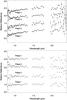 |
Fig. 2 Top panel: the four spectra corresponding to the four rotational phases, shifted by 0.5 in relative reflectance for clarity. Bottom panel: ratio between the four spectra and the average of all of them, also in this case shifted by 0.5 in relative reflectance. |
After analyzing the small variation among all the pairs of each standard, we averaged all of them and used the resulting spectrum of each solar analog to extract the relative reflectance of the target in the four rotational phases. In the top panel of Fig. 2, we show the four final scaled reflectances normalized to unity at 1.6 μm and shifted by 0.5 in relative reflectance for clarity. We do not show the values around the two large telluric bands (1.35−1.46 and 1.82−1.96 μm) because the S/N is very low, and the difference between the spectrum of the object and those of the solar analogs could introduce false features even in rather stable atmospheric conditions.
3. Analysis of the spectra
In comparing the four spectra, we first note that they are all similar within the S/N (Fig. 2 top panel). This is clearest in Fig. 2 (bottom panel), where we show the ratio between each of the spectra and the average of all of them, all of them showing a deviation from unity lower than 2σ. We see that all the spectra are reddish (Fig. 2, top panel) signaling the presence on the surface of Varuna of materials that are more absorbent at the shorter wavelengths. Moreover, the four spectra display an absorption band centered at 2.0 μm, where the water ice has a deep band. As suggested in Licandro et al. (2001), the low depth of the 2.0 μm band and the non-detection of the water-ice band at 1.5 μm suggest that the fraction of water ice in the surface is not high (see Sect. 4). These results are consistent regardless how we define the four phases.
To quantify any possible variation in the slope with the rotation phase, we computed, for each spectrum, the normalized reflectivity gradient S′ [%/1000 Å] in the 0.8−1.8 μm range, where the continuum can be fitted by a straight line (Jewitt, 2002). Results are shown in Table 2. The errors in this table are computed from the fit, taking the dispersion of data in relative reflectance into account. However, as mentioned in the previous section, the systematic errors introduced in the slope are not smaller than 0.65%/1000 Å. Hereafter we use this value for all measurement except those for which the computed errors are larger. The S′ values obtained indicate that the slope does not vary with the rotation within the errors.
Considering the similarity of the four spectra corresponding to the four phases, both in the slope and in the presence of the water ice absorption band, we finally combined them to increase the S/N, obtaining an average spectrum for Varuna with S/N of ~35 in the H band. The resulting spectrum of Varuna is shown in Fig. 3. The average spectrum has a normalized reflectivity gradient of S′ = 2.94 ± 0.65%/1000 Å in the 0.8−1.8 μm range, and a water ice absorption band at 2.0 μm with a depth D = 1−Rb/Rc = 21.0 ± 6.6%, where Rb is the reflectance in the center of the band, and Rc the reflectance of the continuum in the same wavelength, calculated by fitting a cubic spline on the left and the righthand sides of the band.
Normalized reflectivity gradient S′ (see text for definition) for the spectra corresponding to the four rotational phases.
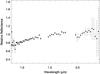 |
Fig. 3 Final averaged spectrum of Varuna normalized at 1.6 μm. |
If we compare our data with the spectrum from Licandro et al. (2001), we find that the slopes of the two spectra are quite different (see Fig. 4). This is probably because Licandro et al. (2001) did not observe a solar analog star. They observed an A0 star for the telluric correction and used the blackbody function of the A0 and G2 star to obtain the relative reflectance.
As can be seen in Fig. 4, the spectrum from Barkume et al. (2008) covers only the H and K range. It is blue and featureless within the S/N. The discrepancy between that spectrum and the one we show in this work cannot be interpreted as indicating surface heterogeneity, given that our spectrum is the average of four almost identical spectra (see Fig. 2 bottom panel) that cover the whole surface of Varuna.
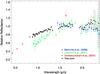 |
Fig. 4 Comparison between our data and data available in the literature. All the spectroscopic data are normalized at 1.6 μm. The photometric data are merged with the spectra in this work in the J band. |
4. Modelization of the reflectance spectrum
4.1. Models with water ice
From the beginning of the study of the surface composition of Centaurs and TNOs, spectra have indicated that they are covered by a mixture of minerals, complex organics, and ices (Barucci et al. 2008; Dalle Ore et al. 2013 and references therein). However, it is not trivial to deconvolve a reflectance spectrum into abundances of the different components because the spectra are complex nonlinear functions of grain size, abundance, and material opacity (Poulet et al. 2002). Nevertheless, models of the scattering of light by particulate surfaces have proven to be useful in studying the surface composition of minor bodies in the solar system.
In this work we have used the Shkuratov theory (Shkuratov et al. 1999) to generate a collection of synthetic spectra that reproduce the overall shape of the spectrum of Varuna. We put special emphasis on the reproduction of the two most representative characteristics of this spectrum, its red slope, and the band at 2.02 μm. These models use the optical constants as input, the relative abundances, and the size of the particles of different materials to compute the albedo of the surface at each wavelength.
It is worthwhile noting here that we compared the synthetic spectra with the reflectance of Varuna using the full visible and NIR wavelength range: the spectrum in the NIR presented in this work and the photometry in the visible (B, V, R, I bands) (Doressoundiram et al. 2007). To give the same weight to the visible part of the data as for the NIR when calculating the goodness of the fit, we generated a synthetic spectrum in the visible from the photometric data, using a spectral resolution that is near to the spectral resolution in the NIR and with a S/N determined by the error associated with the photometric colors.
As a first step, we ran a series of models with different number of components considering materials that are good candidates to be part of the surface of minor icy bodies: complex organics (Triton, Titan, and Ice tholins), olivines, and pyroxenes with different content of magnesium and iron, water ice, amorphous carbon (see Table 1 from Emery & Brown 2004 for the characteristics of the optical constants of silicates, organics, and carbons; Warren, 1984 for the constants of water ice).
We first inspected the fits by eye and find that all the models that reproduce the spectra better include olivine, pyroxene (with a low amount of iron, 20%), triton tholin, amorphous carbon, and water ice. Based on this approximation we decided to use a five-component model mixing these materials as an intimate mixture (salt-and-pepper).
As a second step, we calculated a grid of models varying the relative abundances of these materials from: 0 to 40% for water ice, 0 to 50% for olivine and pyroxene, 0 to 30% for triton tholin, and 0 to 70% for amorphous carbon, with a step of 10% for all of them. We also varied the size of the particles around the best values suggested by the models on the first step: 5 to 23 μm, with a step of 3, for water ice; 50 to 200 μm, with a step of 50 μm, for the olivine and pyroxene, and 3 to 15 μm, with a step of 3, for the tholins. We used a fixed size of 100 μm for the carbon, since the dependance of the reflectance of these dark materials with the particle diameter is insignificant (Fig. 4 from Emery & Brown 2004). The details of the optical constants used in this model are included in Table 3.
Details of the materials used in the best-fit model with water ice.
Finally, we ranked the models using the χ2 value, always using the estimated value for the albedo in the visible as a constraint ( , Lellouch et al. 2013).
The best model in this step consists of an intimate mixture of 25% water ice (17 μm), 15% olivine (50 μm), 10% pyroxene (50 μm), 35% tholin (6 μm) and 15% carbon. The albedo of this model is 10.7%, compatible with value estimated in Lellouch et al. (2013). The amount of water ice resulting from our theoretical model (25%) is consistent with previous results (Licandro et al. 2001) that have suggested that water ice could be present on the surface of Varuna, even if the amount might not be very abundant. The model and spectrum are shown in Fig. 5.
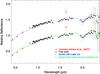 |
Fig. 5 Final spectrum of Varuna together with two models. These models include water ice, silicates, organics, and amorphous carbon (top) and water and methane ice, silicates, organics, and amorphous carbon (bottom). |
This composition is typical of objects covered by a mantle formed by a mixture of silicates, processed materials (complex organics), and water ice. Water ice’s lifetime on the surface of these Centaurs and TNOs is comparable to the age of the solar system, so it could be primordial. No refreshing mechanism is needed in this case to explain the surface composition of this Varuna.
4.2. Models with methane ice
Some of the large TNOs (Makemake, Licandro et al. 2006a; Eris, Brown et al. 2005; Licandro et al. 2006c; Pluto, Cruikshank et al. 1976) are covered by large amounts of methane and other volatiles. The molecule of methane ice is optically very active, so although the surface of these bodies may not be dominated by this material, their visible and NIR spectra are dominated by absorption bands caused by the molecules of methane ice. Other medium-size TNOs have surfaces that contain or could contain a certain amount of light hydrocarbons such as methane ice (e.g., Quaoar, Schaller et al. 2007b; 2007 OR10, Brown et al. 2011). However, this ice is not expected to be common on the surface of most of the TNOs since their temperatures are high enough and masses low enough that all the volatiles would have been removed from the surface on solar system timescales (Schaller & Brown 2007a; Brown et al. 2012a).
Because of its mass and distance from the Sun, Varuna is expected to have already lost all its original inventory of methane ice from the surface; however, some fresh methane could have been exposed to the surface by collisions strong enough to break the mantle and expose fresh material from the interior of the body. This mechanism has been suggested as a mechanism for refreshing the surface of TNOs with fresh materials from the interior of the bodies.
To investigate whether methane ice could be present on the surface of Varuna we ran a final test. We turn our final five-component model into a six-component model, slightly changing the relative abundances to accommodate some methane. We used the optical constants of methane ice at 40 K from Grundy et al. (2002). That we do not see any of the stronger absorption bands in the wavelength range covered by our data (e.g., the 2ν3 transition at 1.67 μm; the ν2 + ν3 + ν2 at 1.72 μm, the ν3 +2ν4 at 1.8 μm or the ν2 + ν3 at 2.21 μm) puts a strong constraint on the abundance and particle size of the methane in our model. Furthermore, small amounts of methane considerably increase the albedo, which reduces the number of possible solutions, given the albedo constraint described above.
We find that the addition of small abundances of methane ice improves (but not strongly affects) the chi-square of our fit. Models could contain up to 10% of methane ice on the surface with a particle size of 20 μm by decreasing the amount of water ice to 20% (20 μm) and the amount of amorphous carbon down to 10%, giving a surface albedo in the visible of 11.3% (Fig. 5). Our best result with methane ice is not unique (spectral models of mineral/ice mixtures are rarely unique, Emery & Brown 2004), but in this case we have some evident restrictions that limit valid ranges for the relative abundances and particle sizes of the different materials. Larger amounts of methane and/or larger particles make the bands (specially those at 1.72 and 2.21 μm) more evident so that they would be detectable in our data. Smaller amounts of silicates or complex organics change the shape of the continuum, and models are also strongly constrained by the depth of the band of water ice at 2.02 μm. Larger amounts of high albedo materials (water ice + methane) would immediately increase the albedo in the visible of model above the valid value.
But how could we explain the presence of methane ice on the surface of an object like Varuna that should be depleted of volatiles? One explanation for any possible CH4 would be is that Varuna suffered from a collision in the past. The mean probability that a object like Varuna suffers from a collision with other TNOs is ⟨ Pi ⟩ = 1.60 × 10⁻²² km-2 yr-1, with medium-impact velocity of ⟨ |U| ⟩ = 2.24 ± 1.08 km s-1. This probability is even higher if we consider collisions between classical TNOs (Dell’Oro et al 2013). These kinds of energetic impacts can bring fresh ices to the surface of a TNO (Gil-Hutton & Brunini 1999), since less energetic impacts only erode the irradiation mantle. As a result of this collision, the irradiation mantle was eroded, and some ice from the interior (methane and water ice) was sublimated and redeposited overall on the surface. The timescale for distributing vapor globally is tens of hours, (Stern 2002), which is longer than the rotational period of Varuna, so the material was globally redeposited over the all surface, offering a possible explanation for the homogeneity. The presence of water and methane ices on the surface, however, is not enough to mask the irradiation mantle, as suggested for other TNOs with a higher content of water ice on the surface, e.g., 1999 TO66 (Brown et al. 1999) and 2002 TX300 (Licandro et al. 2006b). According to Gil-Hutton et al. (2009) thin layers of ices (~10−100 μm) are not able to mask an irradiation mantle below them.
5. Conclusions
We observed Varuna during two consecutive nights, covering twice the rotational period (~6.34 h). We show four averaged relative reflectance spectra (0.8−2.4 μm), each of them corresponding to a fourth of the rotation. After comparing their features (slope and absorption bands), we do not find any indication of surface heterogeneity within the S/N of our data (higher than the S/N of previously published spectra). All our spectra show a reddish slope with an S′ ranging from 2.95 ± 0.31 to 3.52 ± 0.16%/1000 Å and an absorption ~2 μm that is indicative of water ice. This absorption was previously detected by Licandro et al. (2001) in a single spectrum of Varuna. The depth and shape of this band is consistent in the four spectra with a medium depth of 21.0 ± 6.6%. In this case, no refreshing mechanism is needed to explain the surface composition of Varuna.
Our fits of the spectral reflectance using models for the scattering of light indicate that Varuna has a processed surface with some ice content, showing that highly processed materials (complex organics) and silicates coexist with water ice. This composition is homogeneous over all the surface of the body on the spatial scale covered by our data. Water ice’s lifetime on the surface of these bodies is comparable to the age of the object, so the ice could be primordial.
Our data do not show any indication of other volatiles (such as methane ice) on the surface, although the S/N is not high enough to discard their presence. In fact, models show that 10% of methane ice with a particle size of 20 μm improves the fit, while still keeping the value of the albedo compatible with the value estimated by Lellouch et al. (2013). The presence of this ice would indicate that Varuna had suffered a recent energetic impact that would be the responsible for breaking up the mantle of silicates and organics and for replenishing of the surface with fresh material from the interior. This kind of impact also results in homogeneous surfaces like the one we observe for Varuna.
More observations in the H and K band, specifically designed to detect methane ice, would be optimum for disentangling the various scenarios for the recent history of Varuna.
Acknowledgments
N.P.A. acknowledges support from the project AYA2011-30106-C02-01 and the Juan de la Cierva Fellowship Programme of MINECO (Spanish Ministry of Economy and Competitiveness). J.L. acknowledges support from the project AYA2012-39115-C03-03 (MINECO). Based on observations made with the Italian Telescopio Nazionale Galileo (TNG) operated on the island of La Palma by the Fundación Galileo Galilei of the INAF (Istituto Nazionale di Astrofisica) at the Spanish Observatorio del Roque de los Muchachos of the Instituto de Astrofísica de Canarias. We want to thank the referee F. de Meo for her valuable comments that improved the manuscript.
References
- Barkume, K. M., Brown, M. E., & Schaller, E. L. 2008, AJ, 135, 55 [NASA ADS] [CrossRef] [Google Scholar]
- Barucci, M. A., Brown, M. E., Emery, J. P., & Merlin, F. 2008, in The Solar System Beyond Neptune (Tucson: Univ. Arizona Press), 143 [Google Scholar]
- Barucci, M. A., Alvarez-Candal, A., Merlin, F., et al. 2011, Icarus, 214, 297 [NASA ADS] [CrossRef] [Google Scholar]
- Brown, M. E. 2012, Ann. Rev. Earth Planet. Sci., 40, 467 [NASA ADS] [CrossRef] [Google Scholar]
- Brown, M. E., Trujillo, C. A., & Rabinowitz, D. L. 2005, ApJ, 635, 97 [Google Scholar]
- Brown, M. E., Burgasser, A. J., & Fraser, W. C. 2011, ApJ, 738, 26 [Google Scholar]
- Brown, M. E., Schaller, E. L., & Fraser, W. C. 2012, AJ, 143, 146 [Google Scholar]
- Brown, R. H., Cruikshank, D. P., & Pendleton, Y. 1999, ApJ, 519, 101 [Google Scholar]
- Colina, L., & Bohlin, R. 1997, AJ, 113, 1138 [NASA ADS] [CrossRef] [Google Scholar]
- Cruikshank, D. P., Pilcher, C. B., & Morrison, D. 1976, Science, 194, 835 [NASA ADS] [Google Scholar]
- Dalle Ore, C. M., Dal le Ore, L. V., Roush, T. L., et al. 2013, Icarus, 222, 307 [NASA ADS] [CrossRef] [Google Scholar]
- Dell’Oro, A., Campo Bagatin, A., Benavidez, P. G., & Alemañ, R. A. 2013, A&A, 558, A95 [NASA ADS] [CrossRef] [EDP Sciences] [Google Scholar]
- Doressoundiram, A., Peixinho, N., Moullet, A., et al. 2007, AJ, 134, 2186 [NASA ADS] [CrossRef] [Google Scholar]
- Dorschner, J., Begemann, B., Henning, T., Jaeger, C., & Mutschke, H. 1995, A&A, 300, 503 [NASA ADS] [Google Scholar]
- Emery, J. P., & Brown, R. H. 2004, Icarus, 170, 131 [NASA ADS] [CrossRef] [Google Scholar]
- Gil-Hutton, R., & Brunini, A. 1999, Planet. Space Sci., 47, 331 [NASA ADS] [CrossRef] [Google Scholar]
- Gil-Hutton, R., Licandro, J., Pinilla-Alonso, N., & Brunetto, R. 2009, A&A, 500, 909 [NASA ADS] [CrossRef] [EDP Sciences] [Google Scholar]
- Grundy, W. M., Schmitt, B., & Quirico, E. 2002, Icarus, 155, 486 [NASA ADS] [CrossRef] [Google Scholar]
- Jewitt, D. C. 2002, AJ, 123, 1039 [NASA ADS] [CrossRef] [Google Scholar]
- Landolt, A. U. 1992, AJ, 104, 340 [NASA ADS] [CrossRef] [Google Scholar]
- Lellouch, E., Santos-Sanz, P., Lacerda, P., et al. 2013, A&A, 557, A60 [NASA ADS] [CrossRef] [EDP Sciences] [Google Scholar]
- Licandro, J., Oliva, E., & Di Martino, M. 2001, A&A, 373, 29 [Google Scholar]
- Licandro, J., Pinilla-Alonso, N., Pedani, M., et al. 2006a, A&A, 445, L35 [NASA ADS] [CrossRef] [EDP Sciences] [Google Scholar]
- Licandro, J., di Fabrizio, L., Pinilla-Alonso, N., de León, J., & Oliva, E. 2006b, A&A, 457, 329 [NASA ADS] [CrossRef] [EDP Sciences] [Google Scholar]
- Licandro, J., Grundy, W. M., Pinilla-Alonso, N., & Leisy, P. 2006c, A&A, 458, L5 [NASA ADS] [CrossRef] [EDP Sciences] [Google Scholar]
- McDonald, G. D., Thompson, W. R., Heinrich, M., Khare, B. N., & Sagan, C. 1994, Icarus, 108, 137 [NASA ADS] [CrossRef] [Google Scholar]
- Poulet, F., Cuzzi, J. N., Cruikshank, D. P., Roush, T., & Dal le Ore, C. M. 2002, Icarus, 160, 313 [Google Scholar]
- Rouleau, F., & Martin, P. G. 1991, ApJ, 377, 526 [NASA ADS] [CrossRef] [Google Scholar]
- Schaller, E. L., & Brown, M. E. 2007a, ApJ, 659, 61 [Google Scholar]
- Schaller, E. L., & Brown, M. E. 2007b, ApJ, 670, 49 [Google Scholar]
- Shkuratov, Y., Starukhina, L., Hoffmann, H., & Arnold, G. 1999, Icarus, 137, 235 [NASA ADS] [CrossRef] [Google Scholar]
- Stern, S. A. 2002, AJ, 124, 2297 [NASA ADS] [CrossRef] [Google Scholar]
- Thirouin, A., Ortiz, J. L., Duffard, R., et al. 2010, A&A, 522, A93 [NASA ADS] [CrossRef] [EDP Sciences] [Google Scholar]
- Warren, S. G. 1984, ApOpt, 23, 1206 [Google Scholar]
All Tables
Date and time (UT) of the observations and total exposure time corresponding to the four rotational phases in which we divided our Varuna data.
Normalized reflectivity gradient S′ (see text for definition) for the spectra corresponding to the four rotational phases.
All Figures
|
Fig. 1 Top panel: spectra of some pairs of the standard stars observed during the night of 2011 January 08 divided by a pair of Landolt (SA) 102−1081 observed at an airmass of 1.25. Bottom panel: same for the night of 2011 January 09 taking a pair of Landolt (SA) 102−1081 at an airmass of 1.41 as a reference. The airmass of each standard is included in the legend and the spectra are shifted by 0.5 in the vertical for clarity. |
| In the text | |
|
Fig. 2 Top panel: the four spectra corresponding to the four rotational phases, shifted by 0.5 in relative reflectance for clarity. Bottom panel: ratio between the four spectra and the average of all of them, also in this case shifted by 0.5 in relative reflectance. |
| In the text | |
|
Fig. 3 Final averaged spectrum of Varuna normalized at 1.6 μm. |
| In the text | |
|
Fig. 4 Comparison between our data and data available in the literature. All the spectroscopic data are normalized at 1.6 μm. The photometric data are merged with the spectra in this work in the J band. |
| In the text | |
|
Fig. 5 Final spectrum of Varuna together with two models. These models include water ice, silicates, organics, and amorphous carbon (top) and water and methane ice, silicates, organics, and amorphous carbon (bottom). |
| In the text | |
Current usage metrics show cumulative count of Article Views (full-text article views including HTML views, PDF and ePub downloads, according to the available data) and Abstracts Views on Vision4Press platform.
Data correspond to usage on the plateform after 2015. The current usage metrics is available 48-96 hours after online publication and is updated daily on week days.
Initial download of the metrics may take a while.