| Issue |
A&A
Volume 561, January 2014
|
|
|---|---|---|
| Article Number | A62 | |
| Number of page(s) | 7 | |
| Section | The Sun | |
| DOI | https://doi.org/10.1051/0004-6361/201322808 | |
| Published online | 23 December 2013 | |
Kelvin-Helmholtz instability of twisted magnetic flux tubes in the solar wind
1
Space Research Institute, Austrian Academy of Sciences,
8042
Graz,
Austria
e-mail:
This email address is being protected from spambots. You need JavaScript enabled to view it.
2
Faculty of Physics, Sofia University, 5 James Bourchier Blvd., 1164
Sofia,
Bulgaria
3
Abastumani Astrophysical Observatory at Ilia State University,
3/5 Cholokashvili
Avenue, 0162
Tbilisi,
Georgia
Received:
7
October
2013
Accepted:
15
November
2013
Abstract
Context. Tangential velocity discontinuity near the boundaries of solar wind magnetic flux tubes results in Kelvin-Helmholtz instability, which might contribute to solar wind turbulence. While the axial magnetic field stabilizes the instability, a small twist in the magnetic field may allow sub-Alfvénic motions to be unstable.
Aims. We aim to study the Kelvin-Helmholtz instability of twisted magnetic flux tubes in the solar wind with different configurations of the external magnetic field.
Methods. We use magnetohydrodynamic equations in cylindrical geometry and derive the dispersion equations governing the dynamics of twisted magnetic flux tubes moving along its axis in the cases of untwisted and twisted external fields. Then, we solve the dispersion equations analytically and numerically and find thresholds for Kelvin-Helmholtz instability in both cases of the external field.
Results. Both analytical and numerical solutions show that the Kelvin-Helmholtz instability is suppressed in the twisted tube by the external axial magnetic field for sub-Alfvénic motions. However, even a small twist in the external magnetic field allows the Kelvin-Helmholtz instability to be developed for any sub-Alfvénic motion. The unstable harmonics correspond to vortices with high azimuthal mode numbers that are carried by the flow.
Conclusions. Twisted magnetic flux tubes can be unstable to Kelvin-Helmholtz instability when they move with small speed relative to the main solar wind stream, then the Kelvin-Helmholtz vortices may significantly contribute to the solar wind turbulence.
Key words: solar wind / Sun: magnetic fields / instabilities / turbulence
© ESO, 2013
1. Introduction
The solar wind plasma is supposed to be composed of individual magnetic flux tubes that are carried from the solar atmosphere by the wind (Bruno et al. 2001; Borovsky 2008). Tangential velocity discontinuity at the tube surface due to the motion of tubes with regards to the solar wind stream leads to the Kelvin-Helmholtz instability (KHI), which can be of importance as Kelvin-Helmholtz (KH) vortices may lead to enhanced magnetohydrodynamic (MHD) turbulence. Observations show that the velocity difference inside and outside the magnetic structures in the solar wind generally is not large, which means that the relative velocity of the tube and mean stream is sub-Alfvénic. While KHI may develop for small velocity discontinuities in hydrodynamic flows (Drazin & Reid 1981), a flow-aligned magnetic field stabilizes sub-Alfvénic flows (Chandrasekhar 1961). Therefore, KHI will be suppressed in tubes moving with sub-Alfvénic speeds with regards to the solar wind. On the other hand, a transverse magnetic field seems to have no effect on the instability (Sen 1963; Ferrari et al. 1981; Cohn 1983; Singh & Talwar 1994), which means that the twisted magnetic tubes may become unstable to KHI even with sub-Alfvénic motions.
Solar wind flux tubes are probably “fossil structures” (i.e., they are carried from the solar atmosphere), then they can generally keep the magnetic topology typical for tubes near the solar surface. Complex photospheric motions stretch and twist the anchored magnetic field, which might lead to the consequent changes of topology at higher regions. The observed rotation of sunspots (Khutsishvili et al. 1998; Brown et al. 2003; Yan & Qu 2007; Zhang et al. 2007) may lead to the twisting of the magnetic field above active regions, which can be observed as twisted loops in the corona (Srivastava et al. 2010). Recent observations of magnetic tornados (Wedemeyer-Böhm et al. 2012; Su et al. 2012; Li et al. 2012) also strongly support the existence of twisted magnetic flux tubes on the Sun. Newly emerged magnetic tubes can also be twisted in the convection zone during the rising phase (Moreno-Insertis & Emonet 1996; Archontis et al. 2004; Murray & Hood 2008; Hood et al. 2009). Therefore, solar magnetic tubes should have been twisted at photospheric, chromospheric, and coronal levels. The helical magnetic flux rope can also be generated during the eruption of coronal mass ejections (CMEs) and transported into interplanetary space (Lynch et al. 2004). The original magnetic flux rope structure is supposed to be deformed during transport through the heliosphere, but the flux rope will still keep its twisted nature (Manchester et al. 2004). Therefore, the solar wind magnetic tubes of all scales generally should be twisted. Twisted magnetic tubes are unstable to kink instability when the twist exceeds a critical value. The critical twist angle is ~70°, which means that the tubes twisted with a larger angle are unstable to the kink instability, therefore they probably cannot reach 1 AU (Zaqarashvili et al. 2013). Twisted magnetic tubes can be observed by in situ vector magnetic field measurements in the solar wind in the context of the force-free field model (Moldwin et al. 2000; Feng et al. 2007; Telloni et al. 2012), or by variation of total (magnetic + thermal) pressure (Zaqarashvili et al. 2013).
Here, we study KHI for the case of twisted magnetic flux tubes moving along their axes with regards to the mean solar wind stream. The twist is assumed to be small enough, therefore the tubes are stable against kink instability. On the other hand, harmonics with a sufficiently high azimuthal mode number m are always unstable to the KHI in the twisted magnetic tubes moving in a nonmagnetic environment (Zaqarashvili et al. 2010). However, the configuration of an external magnetic field, which stabilizes KHI for sub-Alfvénic flows, is very important. If the magnetic tubes move along the Parker spiral, then the external magnetic field is axial and KHI will be suppressed. However, if the tubes move at an angle to the Parker spiral, then the external magnetic field will have a transverse component, which may allow KHI for sub-Alfvénic motions. In order to study the influence of the transverse component of the external magnetic field on KHI, we consider a small twist in the external magnetic field in cylindrical geometry, so that both the tube and external magnetic fields are stable for the kink instability. To emphasis the role of the transverse component of the external magnetic field, we consider external untwisted and twisted magnetic fields separately and derive KHI thresholds for both cases.
The paper is organized as follows. In Sect. 2, we consider the formulation of the problem and derive the solutions governing the plasma dynamics inside and outside the twisted tubes separately for untwisted and twisted external magnetic fields. In Sect. 3, we derive the dispersion equations of tube dynamics for untwisted and twisted external fields through boundary conditions at the tube surface. In Sect. 4, we solve the dispersion equations both, analytically and numerically, and derive the instability thresholds for KHI. Discussions of the problem and a conclusion are presented in the last, fifth, section.
2. Formulation of the problem and main solutions
We consider a magnetic flux tube with radius a embedded in a magnetized
environment. We use a cylindrical coordinate system (r,φ,z) and assume that
the magnetic field has the following form:
B = (0,Bφ(r),Bz(r)).
The unperturbed magnetic field and pressure satisfy the pressure balance condition
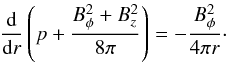 (1)We consider that
the tube moves along the axial direction with regards to the surrounding medium, hence the
flow profile inside the tube is
U = (0,0,U). In general,
U can be a function of r, but we consider the simplest
homogeneous case. No mass flow is considered outside the tube, which means that we are in
the frame co-moving with the solar wind stream.
(1)We consider that
the tube moves along the axial direction with regards to the surrounding medium, hence the
flow profile inside the tube is
U = (0,0,U). In general,
U can be a function of r, but we consider the simplest
homogeneous case. No mass flow is considered outside the tube, which means that we are in
the frame co-moving with the solar wind stream.
As the unperturbed parameters depend on the r coordinate only, the
perturbations can be Fourier analyzed with
exp [ i(mφ + kzz − ωt) ].
The equation governing the incompressible dynamics of the plasma is (Goossens et al. 1992) ![Mathematical equation: \begin{equation} {{\mathrm{d}^2 p_\mathrm{t}}\over {\mathrm{d} r^2}} \!+ \!\left[{{C_3}\over {r D}}{{\mathrm{d} }\over {\mathrm{d} r}}\left ( {{r D}\over {C_3}}\right ) \right ]{{\mathrm{d} p_\mathrm{t}}\over {\mathrm{d} r}} \!+\! \left[{{C_3}\over r D}{{\mathrm{d} }\over {\mathrm{d} r}}\left( {{r C_1}\over {C_3}}\right) \!+\! {{C_2C_3\!-\!C^2_1}\over {D^2}}\right]p_\mathrm{t} = 0,\label{general} \end{equation}](/articles/aa/full_html/2014/01/aa22808-13/aa22808-13-eq12.png) (2)where
(2)where
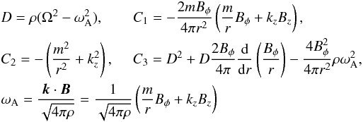 (3)is
the Alfvén frequency,
(3)is
the Alfvén frequency, 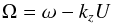 (4)is the Doppler-shifted
frequency, and pt is the total (hydrostatic + magnetic)
perturbed pressure. Radial displacement ξr is
expressed through the total pressure as
(4)is the Doppler-shifted
frequency, and pt is the total (hydrostatic + magnetic)
perturbed pressure. Radial displacement ξr is
expressed through the total pressure as 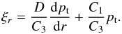 (5)The solution to this
equation depends on the magnetic field and density profiles. Magnetic fields inside and
outside the tube are denoted as Bi and
Be, respectively, while the corresponding
densities are ρi and ρe. To obtain
the dispersion relation of oscillations, we find the solutions inside and outside the tube
and then merge the solutions at the tube boundary through boundary conditions.
(5)The solution to this
equation depends on the magnetic field and density profiles. Magnetic fields inside and
outside the tube are denoted as Bi and
Be, respectively, while the corresponding
densities are ρi and ρe. To obtain
the dispersion relation of oscillations, we find the solutions inside and outside the tube
and then merge the solutions at the tube boundary through boundary conditions.
2.1. Solutions inside the tube
We consider a magnetic flux tube with homogeneous density ρi
and uniform twist, i.e.,  (6)where
A is a constant.
(6)where
A is a constant.
In this case, Eq. (2) reduces to the
modified Bessel equation ![Mathematical equation: \begin{equation} \label{inside} {{\mathrm{d}^2 p_\mathrm{t}}\over {\mathrm{d} r^2}}+{1\over r}{{\mathrm{d} p_\mathrm{t}}\over {\mathrm{d} r}}-\left [{{m^2}\over {r^2}} + m^2_\mathrm{i}\right ]p_\mathrm{t} = 0, \end{equation}](/articles/aa/full_html/2014/01/aa22808-13/aa22808-13-eq25.png) (7)where
(7)where ![Mathematical equation: \begin{equation} \label{m0} m^2_\mathrm{i} = k_z^2 \left[ 1-{{4A^2\omega^2_\mathrm{Ai}}\over {4\pi \rho_\mathrm{i} \left (\Omega^2 - \omega^2_\mathrm{Ai}\right )^2}} \right],\qquad \omega_\mathrm{Ai} = {{mA + k_z B_{\mathrm{i}z}}\over {\sqrt{4\pi \rho_\mathrm{i}}}}\cdot \end{equation}](/articles/aa/full_html/2014/01/aa22808-13/aa22808-13-eq26.png) (8)A similar equation has
been obtained by Dungey & Loughhead (1954)
and Bennett et al. (1999) in the absence of flow,
i.e., for U = 0.
(8)A similar equation has
been obtained by Dungey & Loughhead (1954)
and Bennett et al. (1999) in the absence of flow,
i.e., for U = 0.
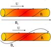 |
Fig. 1 Twisted magnetic tube in two different configurations of external magnetic field: untwisted field (upper panel) and twisted field (lower panel). The tube moves along its axis with constant velocity, U, in both cases. |
The solution bounded at the tube axis is  (9)where
Im is the modified Bessel function of order
m and ai is a constant. Transverse
displacement can be written using Eq. (5)
as
(9)where
Im is the modified Bessel function of order
m and ai is a constant. Transverse
displacement can be written using Eq. (5)
as  (10)where the prime
sign, ′, means a differentiation by the Bessel function argument.
(10)where the prime
sign, ′, means a differentiation by the Bessel function argument.
2.2. Solutions outside the tube
Outside the tube we consider two different configurations of the magnetic field: untwisted (Fig. 1, upper panel) and twisted (Fig. 1, lower panel).
2.2.1. Solution in the presence of the external untwisted magnetic field
In this case, we consider the homogeneous density, ρe, and
the homogenous external untwisted magnetic field of the form  (11)The total
pressure perturbation outside the tube is governed by the same Bessel equation as Eq.
(7), but
(11)The total
pressure perturbation outside the tube is governed by the same Bessel equation as Eq.
(7), but
 is replaced
by
is replaced
by  . The
solution bounded at infinity is
. The
solution bounded at infinity is  (12)where
Km is the modified Bessel function of
order m and ae is a constant.
(12)where
Km is the modified Bessel function of
order m and ae is a constant.
Transverse displacement can be written as  (13)where, as before the
prime sign, ′, means a differentiation by the Bessel function argument and
(13)where, as before the
prime sign, ′, means a differentiation by the Bessel function argument and
 (14)
(14)
2.2.2. Solution in the presence of the external twisted magnetic field
In this case, we consider the external twisted magnetic field of the form 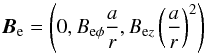 (15)and
the density with the form
ρ = ρe(a / r)4
so that the Alfvén frequency
(15)and
the density with the form
ρ = ρe(a / r)4
so that the Alfvén frequency 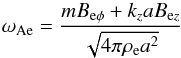 (16)is
constant, which allows us to find an analytical solution of governing equation. The
total pressure perturbation outside the tube is governed by the Bessel-type equation
(16)is
constant, which allows us to find an analytical solution of governing equation. The
total pressure perturbation outside the tube is governed by the Bessel-type equation
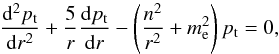 (17)where
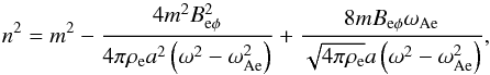 (18)and
  (19)A solution to this
equation bounded at infinity is
(19)A solution to this
equation bounded at infinity is  (20)where
 (21)and
ae is a constant.
(21)and
ae is a constant.
Transverse displacement can be written as  (22)
(22)
3. Dispersion equations
Merging the solutions, i.e., Eqs. (9),
(10), (12), (13), (20), and (22), at the tube surface, r = a, leads
to the dispersion equations governing the dynamics of magnetic tube. In the following we
always consider positive kz. The boundary
conditions at the tube surface are the continuity of Lagrangian displacement and total
Lagrangian pressure (Dungey & Loughhead 1954;
Bennett et al. 1999), i.e., ![Mathematical equation: \begin{equation} \label{boundary1} [\xi_r]_{a} = 0 \end{equation}](/articles/aa/full_html/2014/01/aa22808-13/aa22808-13-eq52.png) (23)and
(23)and ![Mathematical equation: \begin{equation} \label{boundary2} \left [p_\mathrm{t} - {{B^2_{\phi}}\over {4\pi a}}\xi_r \right]_{a} = 0. \end{equation}](/articles/aa/full_html/2014/01/aa22808-13/aa22808-13-eq53.png) (24)Using these conditions, we
can derive the dispersion equations governing the oscillations of moving twisted magnetic
tube in both, untwisted and twisted external magnetic fields.
(24)Using these conditions, we
can derive the dispersion equations governing the oscillations of moving twisted magnetic
tube in both, untwisted and twisted external magnetic fields.
3.1. Dispersion equation for the external untwisted magnetic field
Using Eqs. (9)–(10) and Eqs. (12)–(13), the
following dispersion relation is obtained:
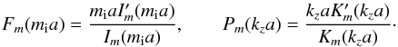
![Mathematical equation: \begin{eqnarray} {{([\omega-k_z U]^2-\omega^2_\mathrm{Ai})F_m(m_\mathrm{i}a)-2mA\omega_\mathrm{Ai}/\!\sqrt{4 \pi \rho_\mathrm{i}}}\over {\rho_\mathrm{i}([\omega-k_z U]^2-\omega^2_\mathrm{Ai})^2-4A^2\omega^2_\mathrm{Ai}/4 \pi}}&=& \nonumber\\ \label{dispersion1} &&{}{{P_{m}(k_z a)}\over {\rho_{\mathrm{e}}(\omega^2-\omega^2_\mathrm{Ae})+A^2P_{m}(k_z a)/4 \pi }}, \end{eqnarray}](/articles/aa/full_html/2014/01/aa22808-13/aa22808-13-eq54.png) (25)where
(25)where
 This
equation is the same as Eq. (13) in Zhelyazkov & Zaqarashvili (2012) with different notations.
This
equation is the same as Eq. (13) in Zhelyazkov & Zaqarashvili (2012) with different notations.
3.2. Dispersion equation for the external twisted magnetic field
Using Eqs. (9)–(10) and Eqs. (20)–(22), the
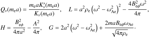
following dispersion relation is obtained: ![Mathematical equation: \begin{eqnarray} {{\left ([\omega-k_z U]^2-\omega^2_\mathrm{Ai} \right )F_m(m_\mathrm{i}a)-2mA\omega_\mathrm{Ai}/\!\sqrt{4 \pi \rho_\mathrm{i}}}\over {\rho_\mathrm{i}\left ([\omega-k_z U]^2 - \omega^2_\mathrm{Ai}\right )^2 - 4A^2\omega^2_\mathrm{Ai}/4 \pi}}&=& \nonumber\\ \label{dispersion2} &&{{a^2\left (\omega^2-\omega^2_\mathrm{Ae}\right )Q_{\nu}(m_\mathrm{e}a)-G}\over {L - H\left [a^2\left (\omega^2-\omega^2_\mathrm{Ae}\right )Q_{\nu}(m_\mathrm{e}a) - G\right ]}}, \end{eqnarray}](/articles/aa/full_html/2014/01/aa22808-13/aa22808-13-eq56.png) (26)where
(26)where
4. Instability criteria
Dispersion Eqs. (25) and (26) govern the dynamics of twisted tubes moving in external untwisted and twisted magnetic fields, respectively. If the frequency, ω, is a complex value, then it indicates an instability process in the system; the real part corresponds to the oscillation and the imaginary part corresponds to the growth rate of instability. Two types of instability may develop in moving twisted tubes: kink instability due to the twist and KHI due to the tangential discontinuity of flow at the tube surface. However, only KHI remains for weakly twisted tubes. Therefore, the condition of complex frequency in Eqs. (25) and (26) serves as the criterion of KHI in weakly twisted tubes.
Equations (25) and (26) are transcendental equations with Bessel functions of complex argument and complex order (for Eq. (26)). We solve the dispersion equations analytically using long wavelength approximation and obtain corresponding analytical instability criteria, then we solve the dispersion equations numerically.
4.1. Instability criterion of twisted magnetic tubes embedded in the untwisted external magnetic field
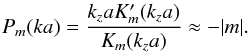
The long wavelength approximation,
kza ≪ 1, yields
mia ≪ 1, therefore we have
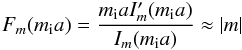 and
and
 Then
Eq. (25) yields the polynomial dispersion
relation
Then
Eq. (25) yields the polynomial dispersion
relation
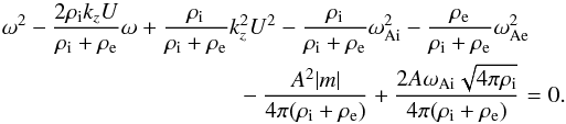 (27)We
consider perturbations with wave vector nearly perpendicular to the magnetic field, i.e.,
k·B ≈ 0, which seem to be
most unstable ones (Pataraya & Zaqarashvili 1995). These modes are pure vortices in the incompressible limit, therefore they
have the strongest growth rate due to KHI. In cylindrical coordinates, this condition is
expressed inside the tube as
(27)We
consider perturbations with wave vector nearly perpendicular to the magnetic field, i.e.,
k·B ≈ 0, which seem to be
most unstable ones (Pataraya & Zaqarashvili 1995). These modes are pure vortices in the incompressible limit, therefore they
have the strongest growth rate due to KHI. In cylindrical coordinates, this condition is
expressed inside the tube as  (28)Then, Eq. (27) is simplified and we find
 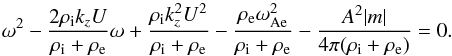 (29)Kelvin-Helmholtz
instability yields the complex frequency, ω, therefore Eq. (29) yields the instability criterion as
(29)Kelvin-Helmholtz
instability yields the complex frequency, ω, therefore Eq. (29) yields the instability criterion as
 (30)where
  (31)is
the Alfvén Mach number and
(31)is
the Alfvén Mach number and  is the Alfvén speed inside the tube.
This criterion means that only super-Alfvénic flows are unstable to KHI in the case of external axial magnetic field. In principle, sub-Alfvénic flows can be also unstable in the case of weak external magnetic field. For Bez = 0, Eq. (30) is transformed into the criterion of KHI in the twisted magnetic tube with nonmagnetic environment (Eq. (28) in Zaqarashvili et al. 2010). But, if the internal and external magnetic fields have similar strengths then KHI only starts for super-Alfvénic motions.
4.2. Instability criterion of twisted magnetic tubes embedded in the twisted external magnetic field
The long wave length approximation,
kza ≪ 1, yields
mia ≪ 1 and
mea ≪ 1, therefore, we have
 and
and
 We
assume that the ratio of azimuthal components of the external and internal magnetic field
is small, i.e.,
Beφ / (aA) ≪ 1
(this yields | ν | ≈ | m |) and consider the
perturbations with
k·Be ≈ 0. Then
Eq. (26) yields the polynomial dispersion
relation
We
assume that the ratio of azimuthal components of the external and internal magnetic field
is small, i.e.,
Beφ / (aA) ≪ 1
(this yields | ν | ≈ | m |) and consider the
perturbations with
k·Be ≈ 0. Then
Eq. (26) yields the polynomial dispersion
relation  (32)We
can further simplify Eq. (32) considering
k·Bi ≈ 0, which
gives
(32)We
can further simplify Eq. (32) considering
k·Bi ≈ 0, which
gives  (33)Then, the
instability criterion is
(33)Then, the
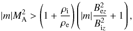
instability criterion is 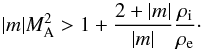 (34)Equation (34) shows that the harmonics with sufficiently
high m are unstable for any value of MA. The
threshold of KHI decreases for higher m. For example, the threshold Mach
number for m = − 1 harmonics is MA ≈ 1.73,
while for m = − 4 harmonics it is reduced to
MA ≈ 0.707
(ρi / ρe = 0.67
is assumed during the estimation). Therefore, the motion of the tube with the speed of
0.71vAi leads to the instability of harmonics with azimuthal
mode numbers
(34)Equation (34) shows that the harmonics with sufficiently
high m are unstable for any value of MA. The
threshold of KHI decreases for higher m. For example, the threshold Mach
number for m = − 1 harmonics is MA ≈ 1.73,
while for m = − 4 harmonics it is reduced to
MA ≈ 0.707
(ρi / ρe = 0.67
is assumed during the estimation). Therefore, the motion of the tube with the speed of
0.71vAi leads to the instability of harmonics with azimuthal
mode numbers  .
The tubes with lower speed will be unstable to higher m harmonics. The
criterion of the KH instability Eq. (34)
is similar to the case of twisted magnetic tube in the nonmagnetic environment
(Zaqarashvili et al. 2010).
.
The tubes with lower speed will be unstable to higher m harmonics. The
criterion of the KH instability Eq. (34)
is similar to the case of twisted magnetic tube in the nonmagnetic environment
(Zaqarashvili et al. 2010).
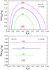 |
Fig. 2 Real (lower panel) and imaginary (upper panel) parts of normalized phase speed, vph / vAi = ω / (kzvAi), vs. normalized wave number kza of m = − 3 unstable harmonics for the external untwisted magnetic field (after numerical solution of dispersion Eq. (25)). Red, green, blue, and magenta lines correspond to Alfvén Mach numbers MA = 1.491,1.5,1.51, and 1.52, respectively. Here, we assume the following parameters: ρi / ρe = 0.67, ε = Biφ / Biz = Aa / Biz = 0.02, and Biz / Bez = 1. |
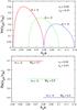 |
Fig. 3 Real (lower panel) and imaginary (upper panel) parts of normalized phase speed, vph / vAi = ω / (kzvAi), vs. normalized wave number kza of unstable harmonics for different values of the Alfvén Mach number (after the numerical solution of the dispersion equation Eq. (26)). Red, green, and blue lines indicate the phase speeds and the growth rates of m = − 2 harmonics for the Alfvén Mach number MA = 0.7, m = − 3 harmonics for the Alfvén Mach number MA = 0.5 and m = − 4 harmonics for the Alfvén Mach number MA = 0.3, respectively. Here, we assume the following parameters: ρi / ρe = 0.67, εi = Biφ / Biz = Aa / Biz = 0.02, εe = Beφ / Bez = 0.01, Biz / Bez = 1. |
5. Numerical solutions of dispersion equations
To check the analytical solutions, we solved the dispersion Eqs. (25) and (26) numerically. The numerical solution of dispersion Eq. (25) shows that all harmonics are stable for sub-Alfvénic flows, MA < 1. Therefore, only super-Alfvénic flows, MA > 1, are unstable in the case of the external untwisted magnetic field. Figure 2 shows m = − 3 unstable harmonics for different values of MA after the solution of Eq. (25). It is seen that the critical Alfvén Mach number equals to 1.491 for m = − 3 harmonics. The analytically estimated critical Mach number (from Eq. (30)) is MA ≈ 1.4907 for m = − 3 harmonics. Hence, there is a very good agreement between the analytical and numerical values. The normalized wave number of unstable harmonics is around kza ≈ 0.06 in Fig. 2, which confirms that the unstable harmonics correspond to the condition k·Bi ≈ 0, which implies kza ≈ − mεi, where εi = Biφ / Biz = Aa / Biz. Both numerical and analytical solutions to Eq. (25) agree with the well-known result that the flow-aligned magnetic field stabilizes KHI.
On the other hand, the numerical solution to Eqs. (26) confirms that there are unstable harmonics with a sufficiently high azimuthal
mode number m for any value of Alfvén Mach number in the case of a twisted
tube with the twisted external magnetic field. Figure 3
shows the unstable harmonics for different values of MA (after
solution of dispersion Eq. (26)). The Alfvén
Mach number MA = 0.7 yields the lowest azimuthal wave number of
the unstable harmonics as m = − 2 and the longitudinal wave number
kza is located in the
interval of 0.04–0.08. Therefore, harmonics with  are unstable for MA = 0.7. The Alfvén Mach number
MA = 0.5 yields the lowest azimuthal wave number as
m = − 3 and the longitudinal wave numbers lay inside the interval of
0.06–0.1. In the same manner, Alfvén Mach number MA = 0.3 yields
the lowest azimuthal wave number and the longitudinal wave number interval as
m = − 4 and 0.08–0.12, respectively. Hence, higher m
harmonics yield a lower Alfvén Mach number in order to become unstable. Numerically
estimated thresholds yield lower values as compared to the analytical instability criterion
Eq. (34). For example, the harmonics with
m = − 3 yield the instability threshold of
MA ≈ 0.8 from Eq. (34), while the numerically obtained threshold is
MA ≈ 0.5. Numerical solutions again confirm that the unstable
harmonics correspond to the condition
k·Bi ≈ 0. We
found that the unstable harmonics with m = − 3 start to be unstable for
εi = 0.02 when
kza = 0.06 as it is expected
(see Fig. 3).
are unstable for MA = 0.7. The Alfvén Mach number
MA = 0.5 yields the lowest azimuthal wave number as
m = − 3 and the longitudinal wave numbers lay inside the interval of
0.06–0.1. In the same manner, Alfvén Mach number MA = 0.3 yields
the lowest azimuthal wave number and the longitudinal wave number interval as
m = − 4 and 0.08–0.12, respectively. Hence, higher m
harmonics yield a lower Alfvén Mach number in order to become unstable. Numerically
estimated thresholds yield lower values as compared to the analytical instability criterion
Eq. (34). For example, the harmonics with
m = − 3 yield the instability threshold of
MA ≈ 0.8 from Eq. (34), while the numerically obtained threshold is
MA ≈ 0.5. Numerical solutions again confirm that the unstable
harmonics correspond to the condition
k·Bi ≈ 0. We
found that the unstable harmonics with m = − 3 start to be unstable for
εi = 0.02 when
kza = 0.06 as it is expected
(see Fig. 3).
Note that the harmonics with negative m and positive εi have identical properties to the harmonics with positive m and negative εi. Figures 2 and 3 show that the phase speed of unstable harmonics corresponds to the flow speed U, which is the speed of the magnetic tube with regards to the solar wind. This result is expected, as k·Bi ≈ 0 condition corresponds to pure vortex solutions. Then, the vortices are carried by the flow and consequently the phase speed of perturbations equals the flow speed.
6. Discussion
Recent observations of KH vortices in solar prominences (Berger et al. 2010; Ryutova et al. 2010) and at boundaries of rising CMEs (Foullon et al. 2011; Ofman & Thompson 2011; Möstl et al. 2013) have resulted in increased interest toward KHI in magnetic flux tubes. The KHI has been studied in the presence of kink oscillations in coronal loops (Terradas et al. 2008; Soler et al. 2010), in twisted magnetic flux tubes with nonmagnetic environment (Zaqarashvili et al. 2010), magnetic tubes with partially ionized plasmas (Soler et al. 2012), in spicules (Zhelyazkov 2012a) and soft X-ray jets (Zhelyazkov 2012b), as well as in photospheric tubes (Zhelyazkov & Zaqarashvili 2012).
Kelvin-Helmholtz vortices can be considered one of the important sources for MHD turbulence in the solar wind. The KHI can be developed by velocity discontinuity at boundaries of magnetic flux tubes owing to the relative motion of the tubes with regards to the solar wind or neighboring tubes. However, the flow-aligned magnetic field may suppress KHI for typical velocity jumps at boundaries of observed magnetic structures in the solar wind, which is generally sub-Alfvénic. The KHI can still survive in the twisted tubes in nonmagnetic environment as the harmonics with sufficiently large m are unstable for any sub-Alfvénic flow along the tubes (Zaqarashvili et al. 2010).
Magnetic structures observed in the solar wind (Bruno et al. 2001; Borovsky 2008), which are believed to be magnetic flux tubes transported from the solar surface, may retain “fossil” properties typical to near-Sun conditions. Magnetic tubes near the solar photosphere, chromosphere, and corona can be twisted for various reasons: during the rising phase along the convection zone (Moreno-Insertis & Emonet 1996; Archontis et al. 2004; Murray & Hood 2008; Hood et al. 2009), by sunspot rotations (Khutsishvili et al. 1998; Brown et al. 2003; Yan & Qu 2007; Zhang et al. 2007), and/or by magnetic tornadoes in the chromosphere and the corona (Wedemeyer-Böhm et al. 2012; Su et al. 2012; Li et al. 2012). Solar prominences are also supposed to be formed in a twisted magnetic field (Priest et al. 1989). Therefore, magnetic flux tubes in the solar wind should be also twisted, which can be detected in situ observations as a variation of the total pressure (Zaqarashvili et al. 2013).
However, just twist inside the magnetic tube is not sufficient for KHI for the case of sub-Alfvénic motions as external flow-aligned magnetic field may stabilize KHI when the vortices start to stretch the magnetic field lines outside the tube. The solar wind magnetic field is generally directed along the Parker spiral, but individual magnetic tubes may move with an angle to the spiral so that the external magnetic field is not necessarily directed along the motion of the tube. Therefore, the configuration of the external magnetic field with regards to the tube motion can be extremely important for the KHI.
Here, we studied KHI instability of the twisted magnetic flux tube moving along its axis in the case of two different configurations of the external magnetic field. First, we assumed that the external magnetic field is directed along the tube axis, so that it is flow aligned. Then, we assumed that the external magnetic field has a small twist, so that the external field has a small angle with the direction of the tube motion. Both, tube and external magnetic fields are only slightly twisted, therefore, they are stable against the kink instability. We solved the incompressible MHD equations in cylindrical coordinates inside and outside the tube and obtained the transcendental dispersion equations through boundary conditions at the tube surface. Then, we solved the dispersion equations analytically in thin flux tube approximation and obtained the instability criteria for both the untwisted and twisted external fields (Eqs. (30) and (34), respectively). We also solved the dispersion equations numerically and found the conditions for KHI. Both, analytical and numerical solutions show that the KHI is suppressed for sub-Alfvénic motions when the twisted tube moves along the Parker spiral, i.e., the external magnetic field is parallel to tube axis and the direction of motion. So our results agree with the already known scenario that the flow aligned magnetic field stabilizes KHI. However, if the external magnetic field has even a very small twist, then the situation is completely changed. We found that the harmonics satisfying the relation k·B ≈ 0 are unstable for any value of the flow. The harmonics with higher m are unstable for sub-Alfvénic motions. The harmonics with wave vectors perpendicular to the magnetic field are in fact pure vortices in the incompressible limit. Therefore, their instability to KHI has a real physical basis as they do not stretch significantly magnetic field lines.
Thus, the analytical and numerical analyses showed that the twisted tubes are always unstable to the KHI when they move in the external twisted magnetic field. This means that the magnetic tubes in the solar wind may excite KH vortices near boundaries. These vortices may be responsible for initial energy in nonlinear cascade leading to MHD turbulence in the solar wind.
7. Conclusions
Twisted magnetic flux tubes can be unstable to KHI when they move with regards to the solar
wind stream. The external axial magnetic field stabilizes KHI, therefore, the tubes moving
along Parker spiral are unstable only for super-Alfvénic motions. The instability criterion
is 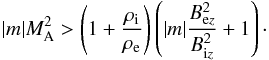 However,
even a slight twist in the external magnetic field leads to KHI for any sub-Alfvénic motion.
Instability criterion in this case is
However,
even a slight twist in the external magnetic field leads to KHI for any sub-Alfvénic motion.
Instability criterion in this case is 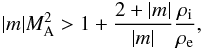 which
shows that the modes with sufficiently large m are always unstable for any
value of the Alfvén Mach number. The unstable harmonics satisfy the relation
k·B ≈ 0, which corresponds
to pure vortices in the incompressible MHD. Therefore, the twisted magnetic tubes moving
with an angle to the Parker spiral may excite KH vortices, which may significantly
contribute to solar wind turbulence.
which
shows that the modes with sufficiently large m are always unstable for any
value of the Alfvén Mach number. The unstable harmonics satisfy the relation
k·B ≈ 0, which corresponds
to pure vortices in the incompressible MHD. Therefore, the twisted magnetic tubes moving
with an angle to the Parker spiral may excite KH vortices, which may significantly
contribute to solar wind turbulence.
Acknowledgments
The work was supported by E.U. collaborative project STORM – 313038. The work of T.Z. was also supported by FP7-PEOPLE-2010-IRSES-269299 project- SOLSPANET, by Shota Rustaveli National Science Foundation grant DI/14/6-310/12 and by the Austrian Fonds zur Förderung der wissenschaftlichen Forschung under project P26181-N27. The work of Z.V. was also supported by the Austrian Fonds zur Förderung der wissenschaftlichen Forschung under project P24740-N27. The work of I.Zh. was supported by the Bulgarian Science Fund under project CSTC/INDIA 05/7.
References
- Archontis, V., Moreno-Insertis, F., Galsgaard, K., Hood, A., & O’Shea, E. 2004, A&A, 426, 1047 [NASA ADS] [CrossRef] [EDP Sciences] [Google Scholar]
- Bennett, K., Roberts, B., & Narain, U. 1999, Sol. Phys., 185, 41 [NASA ADS] [CrossRef] [Google Scholar]
- Berger, T. E., Slater, G., Hurlburt, N., et al. 2010, ApJ, 716, 1288 [NASA ADS] [CrossRef] [Google Scholar]
- Borovsky, J. E. 2008, J. Geophys. Res., 113, A08110 [NASA ADS] [Google Scholar]
- Brown, D. S., Nightingale, R. W., Alexander, D., et al. 2003, Sol. Phys., 216, 79 [NASA ADS] [CrossRef] [Google Scholar]
- Bruno, R., Carbone, V., Veltri, P., Pietropaolo, E., & Bavassano, B. 2001, Planet Space Sci., 49, 1201 [NASA ADS] [CrossRef] [Google Scholar]
- Chandrasekhar, S. 1961, Hydrodynamic and Hydromagnetic Stability (Oxford: Clarendon Press) [Google Scholar]
- Cohn, H. 1983, ApJ, 269, 500 [NASA ADS] [CrossRef] [Google Scholar]
- Drazin, P. G., & Reid, W. H. 1981, Hydrodynamic Stability (Cambridge: Cambridge University Press) [Google Scholar]
- Dungey, J. W., & Loughhead, R. E. 1954, Austr. J. Phys., 7, 5 [NASA ADS] [CrossRef] [Google Scholar]
- Feng, H. Q., Wu, D. J., & Chao, J. K. 2007, J. Geophys. Res., 112, A02102 [Google Scholar]
- Ferrari, A., Trussoni, E., & Zaninetti, L. 1981, MNRAS, 196, 1051 [NASA ADS] [Google Scholar]
- Foullon, C., Verwichte, E., Nakariakov, V. M., Nykyri, K., & Farrugia, C. J. 2011, ApJ, 729, L8 [NASA ADS] [CrossRef] [Google Scholar]
- Goossens, M., Hollweg, J. V., & Sakurai, T. 1992, Sol. Phys., 138, 223 [Google Scholar]
- Hood, A. W., Archontis, V., Galsgaard, K., & Moreno-Insertis, F. 2009, A&A, 503, 999 [NASA ADS] [CrossRef] [EDP Sciences] [Google Scholar]
- Khutsishvili, E., Kvernadze, T., & Sikharulidze, M. 1998, Sol. Phys., 178, 271 [NASA ADS] [CrossRef] [Google Scholar]
- Li, X., Morgan, H., Leonard, D., & Jeska, L. 2012, ApJ, 752, L22 [NASA ADS] [CrossRef] [EDP Sciences] [Google Scholar]
- Lynch, B. J., Antiochos, S. K., MacNeice, P. J., Zurbuchen, T. H., & Fisk, L. A. 2004, ApJ, 617, 589 [NASA ADS] [CrossRef] [Google Scholar]
- Manchester, W. B., Gombosi, T. I., Roussev, I., et al. 2004, J. Geophys. Res., 109, A01102 [NASA ADS] [Google Scholar]
- Moldwin, M. B., Ford, S., Lepping, R., Slavin, J., & Szabo, A. 2000, Geophys. Res. Lett., 27, 57 [NASA ADS] [CrossRef] [Google Scholar]
- Moreno-Insertis, F., & Emonet, T. 1996, ApJ, 472, L53 [NASA ADS] [CrossRef] [Google Scholar]
- Möstl, U. V., Temmer, M., & Veronig, A. M. 2013, ApJ, 766, L12 [NASA ADS] [CrossRef] [Google Scholar]
- Murray, M. J., & Hood, A. W. 2008, A&A, 479, 567 [NASA ADS] [CrossRef] [EDP Sciences] [Google Scholar]
- Ofman, L., & Thompson, B. J. 2011, ApJ, 734, L11 [NASA ADS] [CrossRef] [Google Scholar]
- Pataraya, A. D., & Zaqarashvili, T. V. 1995, Sol. Phys., 157, 31 [NASA ADS] [CrossRef] [Google Scholar]
- Priest, E. R., Hood, A. W., & Anzer, U. 1989, ApJ, 344, 1010 [NASA ADS] [CrossRef] [Google Scholar]
- Ryutova, M., Berger, T., Frank, Z., Tarbell, T., & d Title, A., Sol. Phys., 267, 75 [Google Scholar]
- Sen, A. K. 1963, Phys. Fluids., 6, 1154 [NASA ADS] [CrossRef] [Google Scholar]
- Singh, A. P., & Talwar, S. P. 1994, Sol. Phys., 149, 331 [NASA ADS] [CrossRef] [Google Scholar]
- Soler, R., Terradas, J., Oliver, R., Ballester, J. L., & Goossens, M. 2010, ApJ, 712, 875 [NASA ADS] [CrossRef] [Google Scholar]
- Soler, R., Díaz, A. J., Ballester, J. L., & Goossens, M. 2012, ApJ, 749, 163, 12 [NASA ADS] [CrossRef] [Google Scholar]
- Srivastava, A. K., Zaqarashvili, T. V., Kumar, P., & Khodachenko, M. L. 2010, ApJ, 715, 292 [NASA ADS] [CrossRef] [Google Scholar]
- Su, Y., Wang, T., Veronig, A., Temmer, M., & Gan, W. 2012, ApJ, 756, L41 [NASA ADS] [CrossRef] [Google Scholar]
- Telloni, D., Bruno, R., D’Amicis, R., Pietropaolo, E., & Carbone, V. 2012, ApJ, 751, 19 [NASA ADS] [CrossRef] [Google Scholar]
- Terradas, J., Andries, J., Goossens, M., et al. 2008, ApJ, 687, L115 [Google Scholar]
- Wedemeyer-Böhm, S., Scullion, E., Steiner, O., et al. 2012, Nature, 486, 505 [NASA ADS] [CrossRef] [PubMed] [Google Scholar]
- Yan, X. L., & Qu, Z. Q. 2007, A&A, 468, 1083 [NASA ADS] [CrossRef] [EDP Sciences] [Google Scholar]
- Zhang, J., Li, L., & Song, Q. 2012, ApJ, 662, L35 [Google Scholar]
- Zhou, G. P., Wang, J. X., Zhang, J., et al. 2006, ApJ, 651, 1238 [NASA ADS] [CrossRef] [Google Scholar]
- Zaqarashvili, T. V., Díaz, A. J., Oliver, R., & Ballester, J. L. 2010, A&A, 516, A84 [NASA ADS] [CrossRef] [EDP Sciences] [Google Scholar]
- Zaqarashvili, T. V., Vörös, Z., Narita, Y., & Bruno, R. 2013, ApJL, submitted [Google Scholar]
- Zhelyazkov, I. 2012a, A&A, 537, A124 [NASA ADS] [CrossRef] [EDP Sciences] [Google Scholar]
- Zhelyazkov, I. 2012b, in Topics in Magnetohydrodynamics, ed. L. Zheng (InTech – Open Access Company), Chap. 6 [Google Scholar]
- Zhelyazkov, I., & Zaqarashvili, T. V. 2012, A&A, 547, A14 [NASA ADS] [CrossRef] [EDP Sciences] [Google Scholar]
All Figures
|
Fig. 1 Twisted magnetic tube in two different configurations of external magnetic field: untwisted field (upper panel) and twisted field (lower panel). The tube moves along its axis with constant velocity, U, in both cases. |
| In the text | |
|
Fig. 2 Real (lower panel) and imaginary (upper panel) parts of normalized phase speed, vph / vAi = ω / (kzvAi), vs. normalized wave number kza of m = − 3 unstable harmonics for the external untwisted magnetic field (after numerical solution of dispersion Eq. (25)). Red, green, blue, and magenta lines correspond to Alfvén Mach numbers MA = 1.491,1.5,1.51, and 1.52, respectively. Here, we assume the following parameters: ρi / ρe = 0.67, ε = Biφ / Biz = Aa / Biz = 0.02, and Biz / Bez = 1. |
| In the text | |
|
Fig. 3 Real (lower panel) and imaginary (upper panel) parts of normalized phase speed, vph / vAi = ω / (kzvAi), vs. normalized wave number kza of unstable harmonics for different values of the Alfvén Mach number (after the numerical solution of the dispersion equation Eq. (26)). Red, green, and blue lines indicate the phase speeds and the growth rates of m = − 2 harmonics for the Alfvén Mach number MA = 0.7, m = − 3 harmonics for the Alfvén Mach number MA = 0.5 and m = − 4 harmonics for the Alfvén Mach number MA = 0.3, respectively. Here, we assume the following parameters: ρi / ρe = 0.67, εi = Biφ / Biz = Aa / Biz = 0.02, εe = Beφ / Bez = 0.01, Biz / Bez = 1. |
| In the text | |
Current usage metrics show cumulative count of Article Views (full-text article views including HTML views, PDF and ePub downloads, according to the available data) and Abstracts Views on Vision4Press platform.
Data correspond to usage on the plateform after 2015. The current usage metrics is available 48-96 hours after online publication and is updated daily on week days.
Initial download of the metrics may take a while.