| Issue |
A&A
Volume 561, January 2014
|
|
|---|---|---|
| Article Number | L7 | |
| Number of page(s) | 4 | |
| Section | Letters | |
| DOI | https://doi.org/10.1051/0004-6361/201322782 | |
| Published online | 06 January 2014 | |
Impact of the frequency dependence of tidal Q on the evolution of planetary systems
1
SYRTE, Observatoire de Paris, UMR 8630 du CNRS, UPMC,
77 Av. Denfert-Rochereau,
75014
Paris,
France
e-mail: This email address is being protected from spambots. You need JavaScript enabled to view it.
; This email address is being protected from spambots. You need JavaScript enabled to view it.
2
Laboratoire AIM Paris-Saclay, CEA/DSM – CNRS – Université Paris
Diderot, IRFU/SAp Centre de
Saclay, 91191
Gif-sur-Yvette Cedex,
France
e-mail:
This email address is being protected from spambots. You need JavaScript enabled to view it.
3
IMCCE, Observatoire de Paris, UMR 8028 du CNRS, UPMC,
77 Av.
Denfert-Rochereau, 75014
Paris,
France
4
LESIA, Observatoire de Paris, CNRS UMR 8109, UPMC, Univ. Paris-Diderot,
5 place
Jules Janssen, 92195
Meudon,
France
Received:
2
October
2013
Accepted:
19
November
2013
Abstract
Context. Tidal dissipation in planets and in stars is one of the key physical mechanisms that drive the evolution of planetary systems.
Aims. Tidal dissipation properties are intrinsically linked to the internal structure and the rheology of the studied celestial bodies. The resulting dependence of the dissipation upon the tidal frequency is strongly different in the cases of solids and fluids.
Methods. We computed the tidal evolution of a two-body coplanar system, using the tidal-quality factor frequency-dependencies appropriate to rocks and to convective fluids.
Results. The ensuing orbital dynamics is smooth or strongly erratic, depending on the way the tidal dissipation depends upon frequency.
Conclusions. We demonstrate the strong impact of the internal structure and of the rheology of the central body on the orbital evolution of the tidal perturber. A smooth frequency-dependence of the tidal dissipation causes a smooth orbital evolution, while a peaked dissipation can produce erratic orbital behaviour.
Key words: celestial mechanics / hydrodynamics / planet-star interactions / planets and satellites: dynamical evolution and stability
© ESO, 2014
1. Introduction and context
Tides are one of the key interactions that drive the evolution of planetary systems. Indeed, because of the friction in the host-star and in the planet interiors, a system evolves either to a stable state of minimum energy, where spins are aligned, orbits circularised, and the rotation of each body is synchronised with the orbital motion, or the perturber tends to spiral into the parent body (Hut 1980). Therefore, understanding and modelling the dissipative mechanisms that convert the kinetic energy of tidally excited velocities and displacements into heat is of great importance. These processes, driven by the complex response of a given body (either a star or a planet) to the gravific perturbation by a close companion, strongly depends on its internal structure and its rheology. Indeed, the tidal dissipation in solid (rocky/icy) planetary layers strongly differs from the dissipation in fluid regions in planets and in stars; the one in rocks and ices is often strong with a smooth dependence on the tidal frequency χ, the one in gas and liquids being generally weaker on average and strongly resonant. Therefore, these properties must be taken into account in the study of the dynamical evolution of planetary systems using celestial mechanics.
To reach this objective, the tidal quality factor Q has been introduced in the literature (Goldreich & Soter 1966). Its definition comes from the evaluation of the tidal torque (Kaula 1964) and the analogy with forced damped oscillators: it evaluates the ratio between the maximum energy stored in the tidal distortion during an orbital period and the energy dissipated by the friction. Indeed, a low value of Q corresponds to a strong dissipation, and vice versa. In this framework, Q can be computed from an ab initio resolution of the dissipative dynamical equations for the tidally excited velocities and displacements in fluid and in solid layers of celestial bodies, respectively (e.g. Henning et al. 2009; Efroimsky 2012; Remus et al. 2012b; Zahn 1977; Ogilvie & Lin 2004, 2007; Remus et al. 2012a). This leads to values of Q that varies smoothly as a function of χ in rocks and ices, while numerous and strong resonances are obtained in fluids. However, in celestial mechanics studies, Q is often assumed to be constant or to scale as χ-1 as a convenient first approach and is evaluated using the scenario for the formation and evolution of planetary systems.
In this work, we show how the dependence of Q on χ impacts this evolution and that it must be taken into account. In Sect. 2, we describe the set-up we studied and the corresponding dynamical equations, which correspond to those adopted by Efroimsky & Lainey (2007), who studied the impact of the rheology of solids on related tidal dissipation and evolution (Sect. 3). In Sect. 4, we study highly resonant tidal dissipation in fluid layers and discuss the strong differences with solids. Finally, we discuss astrophysical consequences for the evolution of planetary systems.
2. Set-up and dynamical equations
2.1. Model
To study the impact of rheology on tidal evolution and of the related variation of
Q as a function of χ, we chose to follow Efroimsky & Lainey (2007). We therefore studied
a two-body coplanar system with a central extended body A with a mass
MA and a mean radius RA, and a
point-mass tidal perturber B of mass MB. In a reference-fixed
frame
ℛA:{A,XA,YA,ZA},
the central body rotates with a spin vector ΩA and the perturber
orbits it. To study a simplified system where we can easily isolate the effect of
rheology, this motion was assumed to be circular. Thus, the position of B is directly
given by the semi-major axis a, which is the distance that separates B
from A in this particular case, and the mean anomaly
 , where
nB is the mean motion and t is the time
coordinate.
, where
nB is the mean motion and t is the time
coordinate.
2.2. Dynamical equations
As recalled in the introduction, the tidal quality factor Q is defined
as the ratio between the maximum energy stored in the tidal distortion during an orbital
period and the energy dissipated by the friction. It is thus directly related to the
rheology of the studied bodies, which generally leads to a dependence of
Q as a function of the tidal frequency
 (1)(e.g. Greenberg 2009; Efroimsky
2012), where ω = ω2200 is the
principal semi-diurnal Fourier tidal mode that corresponds to the frequency of the
perturbation in the frame that rotates with the perturber. This friction induces a
geometrical angle δ(χ) between the directions of the
tidal bulge and of the line of centres1
(1)(e.g. Greenberg 2009; Efroimsky
2012), where ω = ω2200 is the
principal semi-diurnal Fourier tidal mode that corresponds to the frequency of the
perturbation in the frame that rotates with the perturber. This friction induces a
geometrical angle δ(χ) between the directions of the
tidal bulge and of the line of centres1![Mathematical equation: \begin{equation} \delta\left(\chi\right)=\frac{1}{2} \chi {\Delta t}\left(\chi\right)=\frac{1}{2}\sin^{-1}\left[Q^{-1}\left(\chi\right)\right], \end{equation}](/articles/aa/full_html/2014/01/aa22782-13/aa22782-13-eq16.png) (2)where we have introduced
the so-called time lag Δt(χ) (see e.g. Hut 1981).
(2)where we have introduced
the so-called time lag Δt(χ) (see e.g. Hut 1981).
This lag induces a net torque that modifies the evolution of the spin of body A (Mathis & Le Poncin-Lafitte 2009) 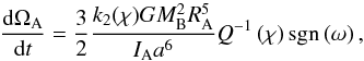 (3)where
IA is the moment of inertia of body A,
k2(χ) is the Love number, and
G is the gravitational constant. The semi-major axis of body B is also
modified (Efroimsky & Lainey 2007)
(3)where
IA is the moment of inertia of body A,
k2(χ) is the Love number, and
G is the gravitational constant. The semi-major axis of body B is also
modified (Efroimsky & Lainey 2007)
 (4)These equations show that
Q-1 has an explicitly linear impact on the evolution of the
system; strong variations of Q-1 thus imply rapid changes for
a and ΩA. Then we took into account the dependence of
Q to χ (e.g. Mathis
& Le Poncin-Lafitte 2009; Efroimsky
& Makarov 2013) to consider the impact of rheological models
straightforwardly.
(4)These equations show that
Q-1 has an explicitly linear impact on the evolution of the
system; strong variations of Q-1 thus imply rapid changes for
a and ΩA. Then we took into account the dependence of
Q to χ (e.g. Mathis
& Le Poncin-Lafitte 2009; Efroimsky
& Makarov 2013) to consider the impact of rheological models
straightforwardly.
3. Solid tides
To solve our problem, we must close it with the choice of a law giving Q (or more generally, k2/Q) as a function of χ. It is common to assume Q to be either constant (e.g. MacDonald 1964) or to scale as χ-1 in the case of a constant tidal time lag (e.g. Hut 1981). However, for solid rocky or icy bodies, Efroimsky & Lainey (2007) suggested to use a power scaling law2: Q = ℰαχα, which has been experimentaly validated for metals and silicates in the laboratory as well as in seismic and geodetic experiments. Here, the empirical parameters α and ℰ are bound to the rheology; α characterises the frequency dependence and takes values between 0.1 and 0.4; ℰ is an integral relaxation parameter, which has the dimension of time and is determined by the internal-friction mechanism that dominates at the frequency χ. Usually, one or another mechanism or group of mechanisms remains dominant across vast bands of frequencies. Over these bands, ℰ may be regarded as constant or almost constant. This law is particularly interesting since it introduces the frequency dependence with only one more parameter than the constant law and remains close to the realistic physics of solids at the same time.
To compute the evolution of a and ΩA with time, we chose to use the numerical code developed by one of us and based on the code ODEX (Hairer et al. 2000). To validate it, we studied the case of the Mars-Phobos system simulated by Efroimsky & Lainey (2007), assuming exactly the same parameters that are summarised in Table 1. The Phobos initial semi-major axis, the initial dissipative time lag, and the constant tidal quality factor are denoted a0, Δt0 and Q.
Numerical values used in the simulation of the Mars-Phobos system.
We note that in this case, the spin of A does not change over time compared to
a because 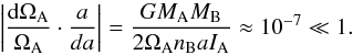 (5)Our results perfectly
reproduce those obtained by Efroimsky & Lainey
(2007). Figure 1 shows the evolution of
a with time for different values of α = −1 (constant
tidal time lag Δt0; e.g. Singer
1968; Mignard 1979), 0 (constant
Q; e.g. Kaula 1964), 0.2, 0.3, and
0.4. These plots highlight the impact of the rheology on the smooth induced evolution of
orbital parameters such as the semi-major axis and on the related life-time of the system.
(5)Our results perfectly
reproduce those obtained by Efroimsky & Lainey
(2007). Figure 1 shows the evolution of
a with time for different values of α = −1 (constant
tidal time lag Δt0; e.g. Singer
1968; Mignard 1979), 0 (constant
Q; e.g. Kaula 1964), 0.2, 0.3, and
0.4. These plots highlight the impact of the rheology on the smooth induced evolution of
orbital parameters such as the semi-major axis and on the related life-time of the system.
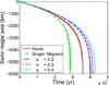 |
Fig. 1 Temporal evolution of the semi-major axis a for a class of tidal models with k2/Q ∝ χ−α and with different values of the parameter α. The abscissa represents time in years, the vertical axis measures the deviation of the semi-major axis from its initial value a0. Our plots serve to compare realistic rheologies (α = 0.2,0.3,0.4) with less physical ones – those with α = 0 (Kaula 1964) and α = −1 (Singer 1968; Mignard 1979). |
4. Tidal dissipation in fluid layers
4.1. Frequency dependence of Q
Revisiting the work by Efroimsky & Lainey (2007) provides a strong basis for exploring the impact of tidal dissipation in fluid bodies. In this section, we therefore chose to study the evolution of a perturber of the mass of Phobos that orbits a hypothetical completely fluid central body with the mass of Mars. Therefore, only the tidal quality factor Q(χ) will change.
In fluid bodies, tidal dissipation is caused by the turbulent viscous friction that acts on the equilibrium tide and on inertial waves, which are driven by the Coriolis acceleration, in convective regions (e.g. Zahn 1977; Ogilvie & Lin 2004, 2007; Remus et al. 2012a), and on thermal and viscous diffusions that act on gravito-inertial waves in stably stratified zones (e.g. Zahn 1977; Ogilvie & Lin 2004, 2007). The excitation of these oscillation eigenmodes by tides then leads to a highly resonant dissipation.
To illustrate our purpose, we consider from now that the central body is completely
convective and rotates rapidly so that 0 ≤ σ ≤ 1, where
σ = χ/(2ΩA), which
generates tidally excited inertial waves. There clearly is a strong difference between the
tidal quality factor adopted before for solid bodies that scale as a smooth power-law of
σ and the one related to inertial waves. Indeed, as demonstrated by
Ogilvie & Lin (2004), using a local
approach, their viscous dissipation is expressed as a sum of corresponding resonant
terms3 (6)where
 and
E = ν/(2ΩAL2)
is the Ekman number of the fluid, ν is the viscosity, and
L a characteristic length; m and n
are the vertical and horizontal wave-vectors of inertial waves, respectively; finally,
fmn and
hmn are the coefficients of the Fourier
series of the excitation. The tidal dissipation is thus a complex set of resonant peaks
depending on the viscosity and on the rotation of the fluid. Since
and
E = ν/(2ΩAL2)
is the Ekman number of the fluid, ν is the viscosity, and
L a characteristic length; m and n
are the vertical and horizontal wave-vectors of inertial waves, respectively; finally,
fmn and
hmn are the coefficients of the Fourier
series of the excitation. The tidal dissipation is thus a complex set of resonant peaks
depending on the viscosity and on the rotation of the fluid. Since
![Mathematical equation: \hbox{$ Q\left(\sigma\right)\propto\left[D\left(\sigma\right)\right]^{-1}$}](/articles/aa/full_html/2014/01/aa22782-13/aa22782-13-eq76.png) ,
we coupled it with the dynamical Eqs. (3),
(4) of our model.
,
we coupled it with the dynamical Eqs. (3),
(4) of our model.
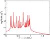 |
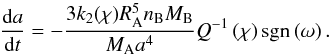
Fig. 2 Resonant tidal dissipation spectrum D resulting from inertial modes as a function of the normalised tidal frequency σ = χ/(2ΩA) assuming Nmax = 5. |
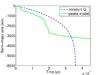 |
Fig. 3 Evolution of the semi-major axis a over time with a Q factor proportional to inertial wave dissipation in fluids (green curve), and with a constant Q factor (blue dashed curve). The abscissa represents time in years, the vertical axis measures the evolution of the semi-major axis from the initial value a0. |
 |
Fig. 4 Evolution of the tidal dissipation and of the semi-major axis with time for different values of lp and Hp, the width at half-height and the height of the studied single resonant damping peak. The grey dotted line corresponding to α = 0.2 is superposed to the continuous green one except at the position of the peak for Q-1. |
4.2. Numerical integration
To evaluate the effects of these resonances on dynamics, we computed the evolution of the
semi-major axis of the orbit with the same parameters as for solid tides, but giving as
input a synthetic  factor written as
  given in Eq. (6). Our fluid is
characterised by its Ekman number, E = 10-5, which is a value
often adopted in the literature for planetary convective layers, and which allows one to
derive a peaked dissipation (see Fig. 2)4. The maximal rank of the sum
(Nmax) was chosen to be relatively low, with
Nmax = 5, to increase the computation speed. Following Ogilvie & Lin (2004), we describe the
excitation with the coefficients
given in Eq. (6). Our fluid is
characterised by its Ekman number, E = 10-5, which is a value
often adopted in the literature for planetary convective layers, and which allows one to
derive a peaked dissipation (see Fig. 2)4. The maximal rank of the sum
(Nmax) was chosen to be relatively low, with
Nmax = 5, to increase the computation speed. Following Ogilvie & Lin (2004), we describe the
excitation with the coefficients 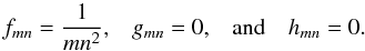 (7)The
simulation clearly shows that, in contrast to solid tides, where the power scaling law
implies a smooth evolution of a, a contrasted Q factor,
that strongly depends on the tidal frequency, enables abrupt changes of a
(see Fig. 3). As the perturber comes nearer to the
central body, its mean motion increases. That is why dissipation varies strongly during
the evolution of the system and, at each time it meets a resonance, there is a jump of
a, which is bounded to the properties of the peak: the higher and wider
the peak, the higher the amplitude of the jump. This is the resonance-locking identified
by Witte & Savonije (1999) in the stellar
case. However, we note that when σ > 1, at the
end of the simulation, the evolution of a becomes smooth again. The
reason for this behaviour is that we are beyond the range of frequencies where inertial
waves are excited. Then, the tidal dissipation is that of the equilibrium tide that
corresponds to the non-resonant background of D observed in Fig. 2. Finally, as demonstrated in Fig. 3, the evolution of a system where the tidal dissipation is caused by
resonant eigenmodes (here the inertial waves) cannot be described properly using models
where Q or Δt are assumed to be constant
(α = 0 and α = −1, respectively).
(7)The
simulation clearly shows that, in contrast to solid tides, where the power scaling law
implies a smooth evolution of a, a contrasted Q factor,
that strongly depends on the tidal frequency, enables abrupt changes of a
(see Fig. 3). As the perturber comes nearer to the
central body, its mean motion increases. That is why dissipation varies strongly during
the evolution of the system and, at each time it meets a resonance, there is a jump of
a, which is bounded to the properties of the peak: the higher and wider
the peak, the higher the amplitude of the jump. This is the resonance-locking identified
by Witte & Savonije (1999) in the stellar
case. However, we note that when σ > 1, at the
end of the simulation, the evolution of a becomes smooth again. The
reason for this behaviour is that we are beyond the range of frequencies where inertial
waves are excited. Then, the tidal dissipation is that of the equilibrium tide that
corresponds to the non-resonant background of D observed in Fig. 2. Finally, as demonstrated in Fig. 3, the evolution of a system where the tidal dissipation is caused by
resonant eigenmodes (here the inertial waves) cannot be described properly using models
where Q or Δt are assumed to be constant
(α = 0 and α = −1, respectively).
4.3. Scaling law
The resonant properties of the tidal dissipation in fluids (see Fig. 2) generate jumps of the value of the semi-major axis a
during the evolution of the system (see Fig. 3). In
this framework, the link between the orbital dynamics and the rheology of the fluid is the
shape of resonances of the viscous dissipation D (see Eq. (6)). A resonance occurs when a term of the sum
in Eq. (6) exceeds all the others. In this
section, our goal is therefore to obtain a scaling law that relates a jump of
a to the height, Hp, and to the width at
half-height, lp, of the corresponding single resonant damping
peak (see Fig. 4) defined as ![Mathematical equation: \begin{equation} Q_{\rm p}^{-1} \left( \sigma \right) = \frac{H_{\rm p}}{ \left[ 4 \left( \sqrt{2} -1 \right) \left(\displaystyle{ \frac{ \sigma - \sigma_{\rm p} }{l_{\rm p}} } \right)^2 +1 \right]^2 }, \label{Qp} \end{equation}](/articles/aa/full_html/2014/01/aa22782-13/aa22782-13-eq94.png) (8)where
σp is the resonant frequency. Then, the dissipation
Q-1 was chosen to be the sum of a smooth background denoted
(8)where
σp is the resonant frequency. Then, the dissipation
Q-1 was chosen to be the sum of a smooth background denoted
 that corresponds to the one studied in Sect. 3, and of a resonant one
 (Eq. (8)), which leads to the following
equation for a using Eq. (4):
(Eq. (8)), which leads to the following
equation for a using Eq. (4): ![Mathematical equation: \begin{equation} \dfrac{{\rm d}a}{{\rm d}t} = - \frac{3 k_2 R_{\rm A}^5 n_{\rm B} M_{\rm B}}{M_{\rm A} a^4 } \left[ Q_0^{-1} \left( \sigma \right) + Q_{\rm p}^{-1} \left( \sigma \right) \right] {\rm sgn} (\omega). \end{equation}](/articles/aa/full_html/2014/01/aa22782-13/aa22782-13-eq98.png) (9)Assuming that the
peak influences the system when the condition
(9)Assuming that the
peak influences the system when the condition  is fullfilled, and that the resulting variation is rapid compared with the mean evolution,
we can derive the amplitude of the jump,
is fullfilled, and that the resulting variation is rapid compared with the mean evolution,
we can derive the amplitude of the jump, ![Mathematical equation: \begin{equation} \frac{\Delta a}{a} \approx \frac{2 l_{\rm p}}{ 3 \sqrt{ \sqrt{2} -1 } \left( 1 + \sigma_{\rm p} \right)} \left[ \sqrt{ \frac{H_{\rm p}}{ Q_0^{-1} \left( \sigma_{\rm p} \right) } } - 1 \right]^{\frac{1}{2}}\cdot \label{SL} \end{equation}](/articles/aa/full_html/2014/01/aa22782-13/aa22782-13-eq100.png) (10)In Fig. 4, we plot the evolution of the semi-major axis for
different values of Hp and lp and
the corresponding dissipation. These graphs illustrate the scaling law (Eq. (10)) by showing that the width of a peak has a
greater impact on a than its height. Moreover, the values of
Δa/a obtained using direct
numerical simulations perfectly match those predicted by Eq. (10). Finally, as
σp, Hp,
lp are directly related to the value of the Eckman number
E = ν/(2ΩAL2)
(cf. Ogilvie & Lin 2004), we see how
(10)In Fig. 4, we plot the evolution of the semi-major axis for
different values of Hp and lp and
the corresponding dissipation. These graphs illustrate the scaling law (Eq. (10)) by showing that the width of a peak has a
greater impact on a than its height. Moreover, the values of
Δa/a obtained using direct
numerical simulations perfectly match those predicted by Eq. (10). Finally, as
σp, Hp,
lp are directly related to the value of the Eckman number
E = ν/(2ΩAL2)
(cf. Ogilvie & Lin 2004), we see how
the orbital dynamics is directly impacted by the fluid rheology and resonances.
5. Conclusions
We examined the impact of the frequency dependence of tidal dissipation in solids and fluids on the orbital evolution of a coplanar two-body system. We showed the strongly different evolutions induced by tides in rocks and by tides exerted on fluid layers where eigenmodes are resonantly excited. A smooth dependence of the tidal dissipation on the tidal frequency drives a smooth orbital evolution, while a peaked dissipation induces an erratic one. In each case, we pointed out the direct impact of the rheology properties on the dynamics of the system. Finally, we showed that it is important to take the dependence of the tidal dissipation on the tidal frequency into account and the important consequences it may have for the evolution of star-planet(s) and planet-moon(s) systems in the solar and exoplanetary systems. In this context, the impact of the frequency dependence of the tidal torque on resonances will be examined in a forthcoming work.
The following identity can be applied only to the m = 2 case (e.g. Efroimsky & Makarov 2013).
Here, we neglect the frequency dependence of the Love number. For realistic materials, the latter approximation is legitimate at a frequency much higher than the inverse Maxwell time.
Global models lead to the same behaviour.
The Eckman number depends on the modelling of the turbulent viscosity (e.g. Ogilvie & Lesur 2012).
Acknowledgments
The authors are grateful to the referee, M. Efroimsky, for his detailed review, which has allowed us to improve the paper. This work was supported by the Programme National de Planétologie (CNRS/INSU), the GRAM specific action (CNRS/INSU-INP, CNES), the Paris Observatory, the Campus Spatial de l’Université Paris Diderot, and the Emergence-UPMC grant (contract number: EME0911). C.L.P.L. and S.M. dedicate this article to Dr. M. Le Poncin.
References
- Efroimsky, M. 2012, ApJ, 746, 150 [NASA ADS] [CrossRef] [Google Scholar]
- Efroimsky, M., & Lainey, V. 2007, J. Geophys. Res. Planets, 112, 12003 [Google Scholar]
- Efroimsky, M., & Makarov, V. V. 2013, ApJ, 764, 26 [NASA ADS] [CrossRef] [Google Scholar]
- Goldreich, P., & Soter, S. 1966, Icarus, 5, 375 [NASA ADS] [CrossRef] [Google Scholar]
- Greenberg, R. 2009, ApJ, 698, L42 [NASA ADS] [CrossRef] [Google Scholar]
- Hairer, E., Nørsett, S., & Wanner, G. 2000, Solving Ordinary Differential Equations I Nonstiff problems, 2nd edn. (Berlin: Springer) [Google Scholar]
- Henning, W. G., O’Connell, R. J., & Sasselov, D. D. 2009, ApJ, 707, 1000 [NASA ADS] [CrossRef] [Google Scholar]
- Hut, P. 1980, A&A, 92, 167 [NASA ADS] [Google Scholar]
- Hut, P. 1981, A&A, 99, 126 [NASA ADS] [Google Scholar]
- Kaula, W. M. 1964, Rev. Geophys. Space Phys., 2, 661 [Google Scholar]
- MacDonald, G. J. F. 1964, Rev. Geophys. Space Phys., 2, 467 [Google Scholar]
- Mathis, S., & Le Poncin-Lafitte, C. 2009, A&A, 497, 889 [NASA ADS] [CrossRef] [EDP Sciences] [Google Scholar]
- Mignard, F. 1979, Moon and Planets, 20, 301 [Google Scholar]
- Ogilvie, G. I., & Lesur, G. 2012, MNRAS, 422, 1975 [NASA ADS] [CrossRef] [Google Scholar]
- Ogilvie, G. I., & Lin, D. N. C. 2004, ApJ, 610, 477 [NASA ADS] [CrossRef] [Google Scholar]
- Ogilvie, G. I., & Lin, D. N. C. 2007, ApJ, 661, 1180 [NASA ADS] [CrossRef] [Google Scholar]
- Remus, F., Mathis, S., & Zahn, J.-P. 2012a, A&A, 544, A132 [NASA ADS] [CrossRef] [EDP Sciences] [Google Scholar]
- Remus, F., Mathis, S., Zahn, J.-P., & Lainey, V. 2012b, A&A, 541, A165 [NASA ADS] [CrossRef] [EDP Sciences] [Google Scholar]
- Singer, S. F. 1968, Geophys. J. Roy. Astron. Soc., 15, 205 [Google Scholar]
- Witte, M. G., & Savonije, G. J. 1999, A&A, 350, 129 [NASA ADS] [Google Scholar]
- Zahn, J.-P. 1977, A&A, 57, 383 [NASA ADS] [Google Scholar]
All Tables
All Figures
|
Fig. 1 Temporal evolution of the semi-major axis a for a class of tidal models with k2/Q ∝ χ−α and with different values of the parameter α. The abscissa represents time in years, the vertical axis measures the deviation of the semi-major axis from its initial value a0. Our plots serve to compare realistic rheologies (α = 0.2,0.3,0.4) with less physical ones – those with α = 0 (Kaula 1964) and α = −1 (Singer 1968; Mignard 1979). |
| In the text | |
|
Fig. 2 Resonant tidal dissipation spectrum D resulting from inertial modes as a function of the normalised tidal frequency σ = χ/(2ΩA) assuming Nmax = 5. |
| In the text | |
|
Fig. 3 Evolution of the semi-major axis a over time with a Q factor proportional to inertial wave dissipation in fluids (green curve), and with a constant Q factor (blue dashed curve). The abscissa represents time in years, the vertical axis measures the evolution of the semi-major axis from the initial value a0. |
| In the text | |
|
Fig. 4 Evolution of the tidal dissipation and of the semi-major axis with time for different values of lp and Hp, the width at half-height and the height of the studied single resonant damping peak. The grey dotted line corresponding to α = 0.2 is superposed to the continuous green one except at the position of the peak for Q-1. |
| In the text | |
Current usage metrics show cumulative count of Article Views (full-text article views including HTML views, PDF and ePub downloads, according to the available data) and Abstracts Views on Vision4Press platform.
Data correspond to usage on the plateform after 2015. The current usage metrics is available 48-96 hours after online publication and is updated daily on week days.
Initial download of the metrics may take a while.