| Issue |
A&A
Volume 561, January 2014
|
|
|---|---|---|
| Article Number | L11 | |
| Number of page(s) | 4 | |
| Section | Letters | |
| DOI | https://doi.org/10.1051/0004-6361/201322671 | |
| Published online | 21 January 2014 | |
First detection of rotational CO line emission in a red giant branch star⋆
Koninklijke Sterrenwacht van België, Ringlaan 3, 1180 Brussel, Belgium
e-mail: This email address is being protected from spambots. You need JavaScript enabled to view it.
Received: 14 September 2013
Accepted: 4 January 2014
Abstract
Context. For stars with initial masses below ~1 M⊙, the mass loss during the first red giant branch (RGB) phase dominates mass loss in the later asymptotic giant branch (AGB) phase. Nevertheless, mass loss on the RGB is still often parameterised by a simple Reimers law in stellar evolution models.
Aims. To try to detect CO thermal emission in a small sample of nearby RGB stars with reliable Hipparcos parallaxes that were shown to have infrared excess in an earlier paper.
Methods. A sample of five stars was observed in the CO J = 2−1 and J = 3−2 lines with the IRAM and APEX telescopes.
Results. One star, the one with the largest mass-loss rate based on the previous analysis of the spectral energy distribution, was detected. The expansion velocity is unexpectedly large at 12 km s-1. The line profile and intensity are compared to the predictions from a molecular line emission code. The standard model predicts a double-peaked profile, while the observations indicate a flatter profile. A model that does fit the data has a much smaller CO envelope (by a factor of 3), and a CO abundance that is two times larger and/or a larger mass-loss rate than the standard model. This could indicate that the phase of large mass loss has only recently started.
Conclusions. The detection of CO in an RGB star with a luminosity of only ~1300 L⊙ and a mass-loss rate as low as a few 10-9M⊙ yr-1 is important and the results also raise new questions. However, ALMA observations are required in order to study the mass-loss process of RGB stars in more detail, both for reasons of sensitivity (6 h of integration in superior weather at IRAM were needed to get a 4σ detection in the object with the largest detection probability), and spatial resolution (to determine the size of the CO envelope).
Key words: circumstellar matter / stars: mass-loss / radio lines: stars
Based on observations made with ESO telescopes at the La Silla Paranal Observatory under programme ID 091.D-0073 (ESO time) and 091.F-9322 (Swedish time). Based on observations with the Atacama Pathfinder EXperiment (APEX) telescope. APEX is a collaboration between the Max Planck Institute for Radio Astronomy, the European Southern Observatory, and the Onsala Space Observatory. Based on observations carried out with the IRAM 30 m Telescope under programme 183-11. IRAM is supported by INSU/CNRS (France), MPG (Germany), and IGN (Spain).
© ESO, 2014
1. Introduction
Stars with initial masses of ≲2.2 M⊙ will go through an evolutionary phase called the first red giant branch (RGB), where stars reach high luminosities (log (L/L⊙) ~ 3). For the lowest initial masses (≲1 M⊙), the total mass lost during the RGB phase dominates that of the AGB (asymptotic giant branch) phase, and therefore it is equally important to understand how this process develops. In stellar evolutionary models, the RGB mass loss is often parameterised by the Reimers law (1975) with a scaling parameter.
In Groenewegen (2012; hereafter G12) a sample of 54 nearby RGB stars was studied. In particular their spectral energy distributions (SEDs) were constructed and fitted with a dust radiative transfer model in order to determine the mass-loss rate. This is complementary to most of the studies on the subject that are based on RGB stars in clusters (see extensive references in G12). Among the 54 stars, 23 stars are found to have a significant infrared excess, which is interpreted as mass loss. In the range 265 < L < 1500L⊙, 22 stars out of 48 experience mass loss, which supports the notion of episodic mass loss.
In the derivation of the (dust) mass-loss rate an expansion velocity (v∞) of 10 km s-1 was adopted. The two main reasons for attempting to detect thermal CO emission is to determine the expansion velocity, and to get an independent estimate of the mass-loss rate. In Sect. 2, the observations are described. In Sect. 3, the results are shown, and interpreted using the model introduced in Sect. 4. The results are discussed in Sect. 5.
RGB sample.
2. Observations
The CO(2−1) observations were obtained on 18−21 February 2012 with the IRAM telescope, located in the Sierra Nevada near Grenada, Spain. Both polarisations of the EMIR E230 receiver (Carter et al. 2012) were tuned to the CO J = 2−1 line and both the VESPA and FTS backends were connected. The results are consistent, and only the results obtained from VESPA are discussed. At that frequency the beam is 10.7′′ (FWHM), and a main-beam efficiency of ηmb = 0.58 is adopted. The weather was at times extremely good (pwv < 0.5 mm), and average system temperatures of Tsys ~ 240 K (Tmb scale) and zenith optical depths τ ~ 0.05 were obtained for some stars. Wobbler switching was used with a throw of 120′′.
The CO(3−2) observations were obtained in service mode on 11 dates between April 14 and July 11, 2013, with the APEX telescope located in the Atacama dessert in Chile. The eXtended bandwidth Fast Fourier Transform Spectrometer (XFFTS) backend (see Klein et al. 2012) was connected to the APEX-2 receiver (Risacher et al. 2006)1 and tuned to the CO J = 3−2 line. At that frequency the beam is 17.3′′ (FWHM), and a main-beam efficiency of ηmb = 0.73 is adopted. The weather was average (pwv 1.0−1.5 mm). Wobbler switching was used with a throw of 50′′.
Five stars were observed from G12, selected because of their visibility and having the highest mass-loss rates. The sources HIP 44126, 53449, 67665, and 88122 were observed with IRAM, and HIP 44126, 53449, and 61658 with APEX. Information on the stars is collected in Table 1. All entries are taken from G12, except the heliocentric radial velocities listed by SIMBAD, that come from Famaey et al. (2009, HIP 88122) and Famaey et al. (2005; the other four stars). The mass-loss rates quoted are derived in G12 based on the modelling of the spectral energy distribution with a dust radiative transfer code and assuming an expansion velocity of 10 km s-1 (a typical expansion velocity, at least for AGB stars) and a dust-to-gas ratio of 1/200.
3. Results
One star is detected, in both transitions. Figure 1 shows the spectra for HIP 53449, for a channel separation of about 2 km s-1. Detailed information on the observation results for all five objects are listed in Table 2.
The J = 2 − 1 line profile is well determined, and can best be described by a flat-topped profile. There appears to be a narrow peak almost exactly at the stellar velocity of − 8.3 km s-1, but this probably fortuitous. In the FTS spectrum the peak is also present but even less clear, and in the original data at the highest velocity resolution (the FTS with a channel separation of 0.25 km s-1, rms noise of 6.5 mK) the peak is not evident. The J = 3 − 2 profile is much noisier and does not provide much insight. In the standard model discussed below a double-peaked profile is expected for both transitions.
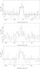 |
Fig. 1 HIP 53449. Top: observed CO(2−1) line profile at a velocity resolution of about 2 km s-1 (histogram), and a typical fit of a shell profile (line, see text). Middle: observed CO(3−2) line profile at a velocity resolution of about 2 km s-1. Bottom: observed CO(3−2) line profile at a lower resolution of about 4 km s-1 (histogram), and a typical fit of a shell profile (line, see text). The velocity scale is heliocentric (the conversion from LSR velocity is done within CLASS). |
Observed results.
A shell-type profile, the one that is used in the CLASS software package2, is fitted to the data: 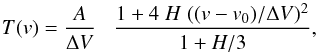 (1)with v0 and ΔV the central velocity, and the full width at zero intensity (both in km s-1); A is the area under the profile (in K km s-1); and H represents the horn-to-centre ratio (− 1 for parabolic optically thick lines, 0 for flat-topped profiles, and a large positive number for double-peaked lines).
The data is still too noisy to allow all parameters to be fitted. For v0 fixed to −8.3 km s-1, and for various fixed line profiles ΔV is found (and then fixed) to be 24 ± 0.7 km s-1 based on the J = 2 − 1 line. The best-fit J = 2 − 1 line profile is near −0.4, so towards a parabolic shape, but the area under the curve and to a lesser extent the peak temperature listed in Table 2 are largely independent of the line shape. Figure 1 shows the fit for a flat-topped profile in the top and bottom panels with the numerical values listed in Table 2. The error bars are derived from a Monte Carlo simulation where the shell-type profile was fitted to 1001 profiles generated from the observed one, but adding the rms noise. It is remarked that Tpeak is not fitted independently but derived from  .
.
4. A model
To help in the interpretation of the observations, the molecular line emission code of Groenewegen (1994a,b) was used. This calculates the line profiles of thermal emission of molecules in an expanding spherically symmetric envelope.
The expansion velocity is set to 12 km s-1. Other parameters (luminosity, stellar radius, effective temperature, grain properties) are taken from G12. In the standard model the mass-loss rate is 5.3 × 10⁻⁹M⊙ yr-1, i.e. the value in Table 1 for an expansion velocity of 12 km s-1 instead of 10 km s-1 and the dust-to-gas ratio is the one assumed in deriving this mass-loss rate from the dust modelling, namely 0.005. The CO abundance relative to H2 is set to fCO = 2 × 10⁻⁴ (Ramstedt et al. 2008). It was verified that cooling by water can be neglected. Following the argumentation in Groenewegen (1994a, near Eq. (16)) water cooling can only be important up to a distance of about 0.19 × 1015 cm for this mass-loss rate and expansion velocity (it will be dissociated to OH farther out), which is about 2 stellar radii, too close to influence the intensity of the CO lower transitions. A velocity law of the form v/v∞ = (1 − R0/r)γ is adopted in Groenewegen (1994a,b), with R0 = 2R∗ and γ = 0.5 in the standard model.
The relative abundance of CO in the envelope is described by the formula proposed by Mamon et al. (1988),  (2)where r1/2 and α depend on Ṁ and v∞ and are tabulated for fCO = 4 × 10⁻⁴ by Mamon et al. (1988), and a fit formula is presented in Stanek et al. (1995). This formulation gives r1/2 = 7 × 1015 cm and α = 1.5. The outer radius of the envelope is set to where the relative CO abundance reaches 1%, or about 2.4 × 1016 cm.
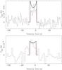 |
Fig. 2 Observed line profiles (histograms) for the J = 2 − 1 (top) and J = 3 − 2 (bottom) transitions. The velocity scale is heliocentric. The standard model is shown as the black solid line, the non-standard model as the red dotted line (see text for details). |
Figure 2 compares the observation to the standard model (the black solid line). The peak intensity and integrated intensity are in remarkable agreement (about 30% for the 2−1 line, and better for the 3−2 line). The obvious discrepancy is in the line shape, which is predicted to be double-peaked, while the observations show otherwise. At the known Hipparcos distance of 119 pc, the value of the outer radius (about 3.5 times r1/2) corresponds to an angular diameter of 27′′, compared to the FWHM beam sizes of 11 and 17′′. The CO shell of the model is resolved by the beams, while the observations suggest otherwise. One way to resolve this discrepancy would be to reduce r1/2, normally implying lower mass-loss rates. The mass-loss rate of a few 10-9M⊙ yr-1 is already smaller than the lowest value listed by Mamon et al. (1 × 10⁻⁸M⊙ yr-1), and in fact for smaller and smaller mass-loss rates a constant value for r1/2 is reached asymptotically which is the value already adopted in the standard model.
The red dotted line in Fig. 2 shows a good fit to the data, reached after some test runs. The parameter r1/2 is reduced to 3 × 1015 cm (outer radius 1 × 1016 cm) to give only a slight double-peaked profile, in better agreement with the data. Making the envelope smaller will result in lower intensities, and this is compensated for by doubling the CO abundance to fCO = 4 × 10⁻⁴, which is still a reasonable value. The same effect could be reached by doubling the mass-loss rate and halving the dust-to-gas ratio. Reducing the envelope size even more would result in a flat-topped and eventually parabolic profile, but would require increasing the CO abundance and/or mass-loss rate as well in order to match the observed intensity.
The shape of the velocity law has little influence on this result. Increasing the velocity gradient by essentially a factor of two far from the star (i.e. changing γ from 0.5 to 1) results in nearly identical line shapes and intensities at the line centre that are lower by 7−10%. Similarly, arbitrarily reducing the kinetic temperature by 20% has very little effect on line shapes and intensities.
5. Discussion
From a sample of 54 nearby RGB stars, 23 of which were shown to have an infrared excess in G12, one star of five observed is detected in CO. It is not easy to distinguish between an RGB and an early-AGB star. Specifically for HIP 53449, the private version of the PARAM tool3 (da Silva et al. 2006), based on the star’s effective temperature, distance, and luminosity, suggests that the star is five times more likely to be on the RGB than the E-AGB (Girardi, priv. comm.)
Even if the star were an E-AGB star and not an RGB star its properties would still be exceptional. Olofsson et al. (2002) present a complitation of the properties of 65 irregular and semiregular oxygen-rich variables based on CO observations. The mass-loss rates range from 2 to 80 × 10-8M⊙ yr-1, with a median value of 20 × 10-8M⊙ yr-1. The object with the lowest mass-loss rate listed is L2 Pup (2 × 10⁻⁸M⊙ yr-1, at 85 pc for an assumed luminosity of 4000 L⊙). Taking its Hipparcos parallax (corresponding to 64 pc) one obtains an improved estimate of ~1 × 10⁻⁸M⊙ yr-1 and a luminosity of 2300 L⊙. This is still considerably more than the ~0.5 × 10⁻⁸M⊙ yr-1 at 1300 L⊙ that is derived here for HIP 53449. The next largest mass-loss rate in the Olofsson et al. sample is BI Car with 3 × 10⁻⁸M⊙ yr-1, but no parallax is known. The next object is θ Aps, where the parallax is in good agreement with the assumed distance, so this object has a mass-loss rate of 4 × 10⁻⁸M⊙ yr-1 at 4000 L⊙. The mass-loss rate in HIP 53449 is extremely low, and at luminosities lower than previously detected.
From simple arguments one expects the peak line intensity to scale with Tpeak ~ Ṁ/D2 (Knapp & Morris 1985). The one star detected has in fact the largest value of this parameter (see the last column of Table 1). The non-detections of the other four objects are then expected given the lower value of Ṁ/D2 and the rms noise in the spectra. This simple comparison assumes that all stars have the same expansion velocity and dust-to-gas ratio, which may not be true.
Nevertheless, the single detection of the star with the largest detection probability (under exceptional weather conditions with a 30 m single-dish telescope) shows that in order to detect mass-loss rates in more objects requires significantly lower rms noise levels, which can only be achieved with ALMA.
Another question that can only be addressed by observing a larger sample is the width of the profile. If it is interpreted as the outflow velocity of an expanding wind, then this velocity (of 12 km s-1) is larger than expected. This value is typical of an average AGB star, while HIP 53449 has a luminosity of only 1300 L⊙.
The high spatial resolution of ALMA observations could address one of the other interesting findings, namely that the
observed line shapes suggest a smaller CO envelope than predicted. New CO photo-dissociation calculations for mass-loss rates lower than considered by Mamon et al. (1988) would be of interest to see if smaller values for r1/2 are found. If the CO envelope is indeed smaller then this could imply that the phase of large mass loss only started recently.
Groenewegen (2012) found that in the range 265 < L < 1500L⊙ only 22 stars out of 48 show mass loss, which supports the notion of episodic mass loss proposed by Origlia et al. (2007). As a test, a model was constructed where the CO abundance was constant with radius, and the outer radius was decreased until the profiles matched the observations. For fCO = 2 × 10⁻⁴ this is 5 × 1015 cm and for fCO = 4 × 10⁻⁴ this is 3 × 1015 cm (or 1.7′′). There is a feedback on the SED modelling because this was originally performed assuming a large outer radius (several 1000 stellar radii) while the CO shell in this test model is only 30−50 stellar radii. Redoing the SED fitting with a smaller outer radius will increase the mass-loss rate estimate to 8.1 × 10⁻⁹M⊙ yr-1, which in turn leads to an even smaller CO shell of 2.5 × 1015 cm (for fCO = 4 × 10⁻⁴). For a velocity of 12 km s-1 a radial distance of (2.5−5) × 1015 cm corresponds to a timescale of 65−130 years. This is a very short timescale, much shorter than the lifetime on the RGB. It would imply that HIP 53449 is caught in the moment where it has just started its phase of large mass loss, which is statistically unlikely.
The observations and the single detection presented here show that detailed studies of the mass-loss process around nearby RGB stars are possible, but require the use of ALMA to increase the number of stars detected and to probe the geometry of the envelope.
Acknowledgments
I would like to thank Leo Girardi (Padova Observatory) for computing the RGB vs. E-AGB probability. This research has made use of the SIMBAD database, operated at CDS, Strasbourg, France.
References
- Carter, M., Lazareff, B., Maier, D., et al. 2012, A&A, 538, A89 [NASA ADS] [CrossRef] [EDP Sciences] [Google Scholar]
- da Silva, L., Girardi, L, Pasquini, L., et al. 2006, A&A, 458, 609 [NASA ADS] [CrossRef] [EDP Sciences] [Google Scholar]
- Famaey, B., Jorissen, A., Luri, X., et al. 2005, A&A, 430, 165 [NASA ADS] [CrossRef] [EDP Sciences] [Google Scholar]
- Famaey, B., Pourbaix, D., Frankowski, A., et al. 2009, A&A, 498, 627 [NASA ADS] [CrossRef] [EDP Sciences] [Google Scholar]
- Groenewegen, M. A. T. 1994a, A&A, 290, 531 [NASA ADS] [Google Scholar]
- Groenewegen, M. A. T. 1994b, A&A, 290, 544 [NASA ADS] [Google Scholar]
- Groenewegen, M. A. T. 2012, A&A, 540, A32 (G12) [NASA ADS] [CrossRef] [EDP Sciences] [Google Scholar]
- Habing, H. J., & Olofsson, H. 2003, Asymptotic Giant Branch Stars (New York: Springer-Verlag) [Google Scholar]
- Klein, B., Hochgürtel, S., Krämer, I., et al. 2012, A&A, 542, L3 [NASA ADS] [CrossRef] [EDP Sciences] [Google Scholar]
- Knapp, G. R., & Morris, M. 1985, ApJ, 292, 640 [NASA ADS] [CrossRef] [Google Scholar]
- Mamon, G. A., Glassgold, A. E., & Huggins, P. J. 1988, ApJ, 328, 797 [NASA ADS] [CrossRef] [Google Scholar]
- Olofsson, H., González Delgado, D., Kerschbaum, F., & Schöier, F. L. 2002, A&A, 391, 1053 [NASA ADS] [CrossRef] [EDP Sciences] [Google Scholar]
- Origlia, L., Rood, R. T., Fabbri, S., et al. 2007, ApJ, 667, L85 [NASA ADS] [CrossRef] [Google Scholar]
- Ramstedt, S., Schöier, F. L., Olofsson, H., & Lundgren, A. A. 2008, A&A, 487, 645 [NASA ADS] [CrossRef] [EDP Sciences] [Google Scholar]
- Reimers, D. 1975, Mem. Soc. Roy. Sci. Liège, 8, 369 [Google Scholar]
- Risacher, C., Vassilev, V., Monje, R., et al. 2006, A&A, 454, L17 [NASA ADS] [CrossRef] [EDP Sciences] [Google Scholar]
- Stanek, K. Z, Knapp, G. R., Young, K., & Phillips, T. G. 1995, ApJS, 100, 169 [NASA ADS] [CrossRef] [Google Scholar]
All Tables
All Figures
|
Fig. 1 HIP 53449. Top: observed CO(2−1) line profile at a velocity resolution of about 2 km s-1 (histogram), and a typical fit of a shell profile (line, see text). Middle: observed CO(3−2) line profile at a velocity resolution of about 2 km s-1. Bottom: observed CO(3−2) line profile at a lower resolution of about 4 km s-1 (histogram), and a typical fit of a shell profile (line, see text). The velocity scale is heliocentric (the conversion from LSR velocity is done within CLASS). |
| In the text | |
|
Fig. 2 Observed line profiles (histograms) for the J = 2 − 1 (top) and J = 3 − 2 (bottom) transitions. The velocity scale is heliocentric. The standard model is shown as the black solid line, the non-standard model as the red dotted line (see text for details). |
| In the text | |
Current usage metrics show cumulative count of Article Views (full-text article views including HTML views, PDF and ePub downloads, according to the available data) and Abstracts Views on Vision4Press platform.
Data correspond to usage on the plateform after 2015. The current usage metrics is available 48-96 hours after online publication and is updated daily on week days.
Initial download of the metrics may take a while.