| Issue |
A&A
Volume 561, January 2014
|
|
|---|---|---|
| Article Number | A88 | |
| Number of page(s) | 7 | |
| Section | Numerical methods and codes | |
| DOI | https://doi.org/10.1051/0004-6361/201322177 | |
| Published online | 07 January 2014 | |
Compressed convolution
1
Department of Physics and AstronomyUniversity College London,
London
WC1E 6BT,
UK
e-mail:
This email address is being protected from spambots. You need JavaScript enabled to view it.
2
Institut d’Astrophysique de Paris, UMR 7095, CNRS - Université
Pierre et Marie Curie (Univ Paris 06), 98 bis blvd Arago, 75014
Paris,
France
3
Departments of Physics and Astronomy, University of Illinois at
Urbana-Champaign, Urbana
IL
61801,
USA
Received:
29
June
2013
Accepted:
11
December
2013
Abstract
We introduce the concept of compressed convolution, a technique to convolve a given data set with a large number of non-orthogonal kernels. In typical applications our technique drastically reduces the effective number of computations. The new method is applicable to convolutions with symmetric and asymmetric kernels and can be easily controlled for an optimal trade-off between speed and accuracy. It is based on linear compression of the collection of kernels into a small number of coefficients in an optimal eigenbasis. The final result can then be decompressed in constant time for each desired convolved output. The method is fully general and suitable for a wide variety of problems. We give explicit examples in the context of simulation challenges for upcoming multi-kilo-detector cosmic microwave background (CMB) missions. For a CMB experiment with detectors with similar beam properties, we demonstrate that the algorithm can decrease the costs of beam convolution by two to three orders of magnitude with negligible loss of accuracy. Likewise, it has the potential to allow the reduction of disk space required to store signal simulations by a similar amount. Applications in other areas of astrophysics and beyond are optimal searches for a large number of templates in noisy data, e.g. from a parametrized family of gravitational wave templates; or calculating convolutions with highly overcomplete wavelet dictionaries, e.g. in methods designed to uncover sparse signal representations.
Key words: methods: data analysis / methods: statistical / methods: numerical / cosmic background radiation
© ESO, 2014
1. Introduction
Convolution is a very common operation in processing pipelines of scientific data sets. For example, in the analysis of cosmic microwave background (CMB) radiation experiments, convolutions are used to improve the detection of point sources (e.g., Tegmark & de Oliveira-Costa 1998; Cayón et al. 2000), in the search for non-Gaussian signals on the basis of wavelets (e.g., Barreiro & Hobson 2001; Martínez-González et al. 2002), during mapmaking (e.g., Tegmark 1997; Natoli et al. 2001), or Wiener filtering (Elsner & Wandelt 2013).
Convolution for data simulation presents similar if not greater challenges: the current and next generations of CMB experiments are nearly photon-noise limited. The only way to reach the sensitivity required to detect and resolve B-modes or to resolve the Sunyaev-Zel’dovich effect of clusters of galaxies over large fractions of sky is to build detector arrays with N ~ 102−104 detectors. Simulating the signal for these experiments requires convolving the same input sky with N different and often quite similar kernels.
In the simplest case, when the convolution kernel is azimuthally symmetric, convolution involves the computation of spherical harmonic transformations. Although highly optimized implementations exist (e.g., libsharp, Reinecke & Seljebotn 2013; the default back end in the popular HEALPix library, Górski et al. 2005), spherical harmonic transformations are numerically expensive and may easily become the bottleneck in data simulation and processing pipelines.
Even more critical is the more realistic setting when the kernels are anisotropic (e.g., when modeling the physical optics of a CMB experiment or when performing edge or ridge detection with curvelets or steerable filters, e.g., Wiaux et al. 2006; McEwen et al. 2007) In this case, the cost of convolution additionally scales with the degree of azimuthal structure in the kernel (Wandelt & Górski 2001) and the convolution output is parametrized in terms of three Euler angles each taking ~L distinct values, where L is the bandlimit of the convolution output. Storing thousands of such objects, one for each beam, requires storage capacity approaching the peta-byte scale.
In this paper, we show that regardless of the details of the convolution problem, or the algorithm used for performing the convolution, the computational costs and storage requirements associated with multiple convolutions can be considerably reduced as long as the set of convolution kernels contains linearly compressible redundancy. Our approach exploits the linearity of the convolution operation to represent the set of convolution kernels in terms of an often much smaller set of optimal basis kernels. We demonstrate that this approach can greatly accelerate several examples taken from CMB data simulation and analysis.
Approaches based on singular value decompositions (SVD) have already proven very successful in observational astronomy to correct imaging data for spatially varying point spread functions (e.g., Lupton et al. 2001; Lauer 2002). Likewise, SVDs have been used to accelerate the search for gravitational wave signatures (e.g., Cannon et al. 2010) using precomputed templates (Jaranowski & Królak 2005). In this paper, we show these methods to be special cases of a more general approach that returns a signal-to-noise eigenbasis that achieves optimal acceleration and compression for a given accuracy goal.
The paper is organized as follows. In Sect. 2, we introduce the mathematical foundations of our method. Using existing spaceborne and ground based CMB experiments as an example, we then analyze the performance of the compressed convolution scheme when applied to the beam convolution problem (Sect. 3). After outlining the scope of our algorithm in Sect. 4, we summarize our findings in Sect. 5.
2. Method
Starting from the defining equation of the convolution integral, we first review the basic
concept of the algorithm. Given a raw data map
d(x), the convolved object (time stream,
map) s(x) is derived by convolution with a
kernel
K(x,y),
 (1)Note
that, without loss of generality, we focus on the convolution of two-dimensional data sets
in this paper.
(1)Note
that, without loss of generality, we focus on the convolution of two-dimensional data sets
in this paper.
2.1. Overview
In practice, a continuous signal is usually measured only on a finite number of discrete
pixels. We therefore approximate the integral in Eq. (1) by a sum in what follows, 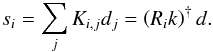 (2)For
our subsequent analysis, we introduced the operator R in the latter
equation such that Rik is
the ith row of the convolution matrix, constructed from the convolution
kernel K.
(2)For
our subsequent analysis, we introduced the operator R in the latter
equation such that Rik is
the ith row of the convolution matrix, constructed from the convolution
kernel K.
For any complete set of basis functions
{ φ1,...,φN },
there exists a unique set of coefficients
{ λ1,...,λN },
such that 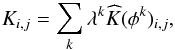 (3)i.e.,
we do a basis transformation of the kernel from the standard basis to the basis given by
the { φk }.
(3)i.e.,
we do a basis transformation of the kernel from the standard basis to the basis given by
the { φk }.
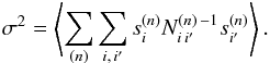
Taking advantage of the linearity of the convolution operation, Eq. (2) can then be transformed to read
 (4)where
the sk are the raw input map convolved with
the kth mode of the basis functions themselves. That is, the final
convolution outputs are now expressed in terms of a weighted sum of individually convolved
input maps with a set of basis kernels.
(4)where
the sk are the raw input map convolved with
the kth mode of the basis functions themselves. That is, the final
convolution outputs are now expressed in terms of a weighted sum of individually convolved
input maps with a set of basis kernels.
We note that for a single convolution operation, the decomposition of the convolution kernel into multiple basis functions in Eq. (4) cannot decrease the numerical costs of the operation. However, potential performance improvements can be realized if multiple convolutions are to be calculated, as we will discuss in the following.
Consider the particular problem where a single raw map d should be
convolved with ntot different convolution kernels, i.e., we
want to compute 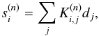 (5)where
we introduced the kernel ID
n ∈ { 1,...,ntot }
as a running index.
(5)where
we introduced the kernel ID
n ∈ { 1,...,ntot }
as a running index.
Applying the kernel decomposition into a common set of basis functions, Eq. (4) now reads 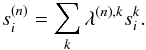 (6)This
finding builds the foundation of our fast algorithm: the numerically expensive convolution
operations are applied only to a limited number of basis modes used in the expansion. The
computational cost is therefore largely independent of the total number of kernels,
ntot, since each individual solution is constructed very
efficiently via a simple linear combination out of a set of precomputed convolution
outputs.
(6)This
finding builds the foundation of our fast algorithm: the numerically expensive convolution
operations are applied only to a limited number of basis modes used in the expansion. The
computational cost is therefore largely independent of the total number of kernels,
ntot, since each individual solution is constructed very
efficiently via a simple linear combination out of a set of precomputed convolution
outputs.
2.2. Optimal kernel expansion
For the kernel decomposition in Eq. (6) to
be useful in practice, we have to restrict the total number of basis modes for which the
convolution is calculated explicitly. To find the optimal expansion, i.e., the basis set
with the smallest number of modes for a predefined truncation error, we first define the
weighted sum of the expected covariance of all the elements of the convolution output
 (7)Here,
we have introduced a real symmetric weighting matrix,
N(n), which allows us to specify what aspects
of the convolved maps we require to be accurate. For the case of convolving to simulate
CMB data, a natural choice for N(n) would be the
noise covariance for the nth channel. It ensures that any given channel
will be simulated at sufficient accuracy and that after the addition of instrumental
noise, the statistics of the resulting simulation are indistinguishable from an exact
simulation.
(7)Here,
we have introduced a real symmetric weighting matrix,
N(n), which allows us to specify what aspects
of the convolved maps we require to be accurate. For the case of convolving to simulate
CMB data, a natural choice for N(n) would be the
noise covariance for the nth channel. It ensures that any given channel
will be simulated at sufficient accuracy and that after the addition of instrumental
noise, the statistics of the resulting simulation are indistinguishable from an exact
simulation.
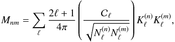
It is now easy to see how to decompose the kernels into a basis such a way as to
concentrate the largest amount of variance in the first basis elements. Define the
Hermitian matrix ![Mathematical equation: \begin{eqnarray} \label{eq:weighted_covariance} M_{nm} &= \left \langle \sum_{i, \, i^{\prime}, \, i^{\prime \prime}} N^{(n) \, -\frac{1}{2}}_{i^\prime \, i} s_i^{(n)} N^{(m) \, -\frac{1}{2}}_{i^{\prime} \, i^{\prime \prime}} s_{i^{\prime \prime}}^{(m)} \right \rangle \nonumber \\ & = \sum_{i, \, i^{\prime}} \left[ \left( N^{(n) \, -\frac{1}{2}} \right)^{\dagger} N^{(m) \, -\frac{1}{2}} \right]_{i \, i^{\prime}} \left( R_{i^{\prime}} k^{(m)} \right) \mathbf{C} \left( R_{i} k^{(n)} \right)^{\dagger} , \end{eqnarray}](/articles/aa/full_html/2014/01/aa22177-13/aa22177-13-eq30.png) (8)where
C is the covariance of the input signal and
(8)where
C is the covariance of the input signal and
 is any matrix such that
 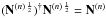 .
.
Then we can rewrite the scalar Eq. (7) as
a matrix trace over the kernel IDs  (9)Since
the matrix in Eq. (9) is Hermitian, its
ordered diagonal elements cannot decrease faster than its ordered eigenvalues by Schur’s
theorem. Finding the eigensystem of M therefore results in the kernel
decomposition that converges faster than any other decomposition to the result of the
direct computation. In other words, the decomposition is optimal because discarding the
eigenmodes with the smallest eigenvalues results in the smallest possible change in the
overall signal power.
(9)Since
the matrix in Eq. (9) is Hermitian, its
ordered diagonal elements cannot decrease faster than its ordered eigenvalues by Schur’s
theorem. Finding the eigensystem of M therefore results in the kernel
decomposition that converges faster than any other decomposition to the result of the
direct computation. In other words, the decomposition is optimal because discarding the
eigenmodes with the smallest eigenvalues results in the smallest possible change in the
overall signal power.
If we denote the eigenvectors of M by
ur, with corresponding eigenvalues
νr, the optimal compression kernel
eigenmodes are given by  , and
the mean square truncation error is the sum of the truncated eigenvalues.
, and
the mean square truncation error is the sum of the truncated eigenvalues.
Considering the CMB case of a convolution on the sphere with azimuthally symmetric
convolution kernels and multipole-dependent diagonal weights,
Nℓ, Eq. (8) simplifies to
 (10)and
Eq. (9) becomes
(10)and
Eq. (9) becomes
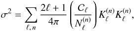 (11)which
clearly shows the signal-to-noise weighting at work.
(11)which
clearly shows the signal-to-noise weighting at work.
Note, that the expression for the variance can be promoted to a matrix in a dual way,
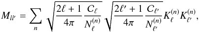 (12)which
gives rise to an alternative way to calculate the optimal compression basis.
(12)which
gives rise to an alternative way to calculate the optimal compression basis.
This dual approach will be computationally more convenient than the other approach if the number of kernels is larger than the number of multipoles in the ℓ-range considered. The resulting compression scheme will be identical in both cases. This is so because both approaches are optimal by Schur’s theorem and each gives a unique answer if none of the eigenvalues are degenerate1.
2.3. Truncation error estimates
In case the kernels are of similar shape, or differ only in regimes that are irrelevant
due to low signal-to-noise, the eigenvalues of the individual modes will decrease quickly.
As a result, we can truncate the expansion in Eq. (6) at nmodes ≪ ntot.
This will induce a mean square truncation in the weighted variance of the convolution
products of  .
.
The error ΔK introduced by the truncation can be calculated for each
kernel explicitly, 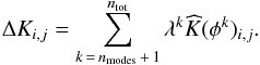 (13)For
the convolution of a data set with power spectrum
(13)For
the convolution of a data set with power spectrum  on the sphere, for example, the mean square error will then amount to
 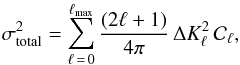 (14)where
ΔKℓ is the expansion of the beam truncation
error into Legendre polynomials.
(14)where
ΔKℓ is the expansion of the beam truncation
error into Legendre polynomials.
2.4. Connection to the SVD
While Eq. (9) provides us with the optimal kernel decomposition, the power spectrum of the data or their noise properties to construct the kernel weights may not necessarily be known in advance. For uniform weightings, N ∝1, and assuming a flat signal power spectrum, the equation simplifies and we obtain the mode expansion from a singular value decomposition of the collection of kernels.
Although not strictly optimal, we note that it is possible to obtain good results with
this simplified approach in practice. To compute the kernel expansion, we reshape the
convolution kernels into one-dimensional arrays of length m and arrange
them into a common matrix T, with size
ntot × m. The singular value decomposition
of this matrix,  (15)computes
the ntot × ntot matrix
U, the ntot × m matrix
D, and the m × m matrix V.
The decomposition then provides us with a set of basis functions, returned in the columns
of V. Their relative importance is indicated by the entries of the diagonal
matrix D, and their individual coefficients λ are stored in
U.
(15)computes
the ntot × ntot matrix
U, the ntot × m matrix
D, and the m × m matrix V.
The decomposition then provides us with a set of basis functions, returned in the columns
of V. Their relative importance is indicated by the entries of the diagonal
matrix D, and their individual coefficients λ are stored in
U.
2.5. Summary
In summary, the individual steps of the algorithm are as follows: we first find the eigenmode decomposition of the set of convolution kernels using either the optimal expansion criterion or a simplified singular value decomposition. Then, we identify the number of modes to retain to comply with the accuracy goal. As a next step, we perform the convolution of the input map for each eigenmode separately. To obtain the final results, we compute the linear combination of the convolved maps with optimal weights for each kernel.
It is worth noting that compressed convolution can never increase the computational time required for convolution, except possibly for some overhead of sub-leading order, attributed to the calculation of the optimal kernel expansion (this computation has to be done only once for a given set of kernels). This can be seen explicitly in the worst case scenario of strictly orthogonal kernels: all modes must be retained and the method becomes equivalent to the brute force approach.
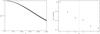 |
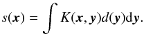
Fig. 1 All six Planck beams at 217 GHz (left panel) have very similar shapes. As a result, the eigenvalues of their singular value decomposition decrease quickly (right panel), allowing half of the modes to be safely discarded. |
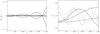 |
Fig. 2 Left panel: retaining the first three out of six
Planck 217 GHz beam eigenmodes allows to reduce the relative
truncation error of all convolution kernels to the order
|
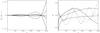 |
Fig. 3 Kernel weights allow for a full control over truncation errors. Same as Fig. 2, but for a
|

3. Application to CMB experiments
After having outlined the basic principle of the algorithm, we now analyze the performance of the method when applied to the beam convolution operation of current CMB experiments.
3.1. Planck
We use the third generation CMB satellite experiment Planck (Planck Collaboration 2011) as a first example to illustrate the application of the algorithm. We make use of the 217 GHz HFI instrument (Planck HFI Core Team 2011) and consider the beam convolution problem of CMB simulations. Azimuthally symmetrized beam functions for the six individual detectors at that frequency are available from the reduced instrument model (Planck Collaboration 2014).
A comparison of the eigenvalues of a singular value decomposition reveals that the beam
shapes are sufficiently similar to be represented with only a limited number of basis
functions (Fig. 1). As shown in Fig. 2, selecting the first three eigenmodes for a
reconstruction is sufficient to represent the beams to an accuracy of the order
 ,
better than the typical precision to which the beams are known.
,
better than the typical precision to which the beams are known.
To illustrate the impact of the weighting scheme, we also show the resulting eigenmodes
using the optimal kernel expansion (Eq. (12)) in Fig. 3. Here, we assumed a white
noise power spectrum,
Nℓ = const., in
combination with a signal covariance of  ,
reflecting the approximate scaling behavior of the CMB power spectrum.
,
reflecting the approximate scaling behavior of the CMB power spectrum.
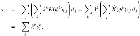
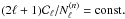
We chose the beam with the largest reconstruction error for an explicit test on simulated CMB signal maps. In Fig. 4, we plot the difference map computed from the brute force beam convolution and the compressed convolution with three eigenmodes. A power spectrum analysis confirms that the truncation induced errors are clearly subdominant on all angular scales.
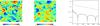 |
Fig. 4 Truncation errors are negligible. Using the kernel with the largest truncation error as worst case scenario, we plot the beam convolved simulated CMB map used in this test of the Planck 217 GHz channels (left panel, we show a 10° × 10° patch). Middle panel: the difference map between the results obtained with the exact convolution and the compressed convolution with three beam modes. Right panel: compared to the fiducial power spectrum of the input map (dashed line), the power spectrum of the difference map is subdominant by a large margin on all angular scales. |
The test demonstrates that the algorithm can be applied straightforwardly to the beam convolution problem. In case of the six Planck 217 GHz detectors, we reduce the number of computationally expensive spherical harmonic transformations by a factor of two. This finding is characteristic for the scope of the algorithm: for a small total number of convolution kernels, the reductions in computational costs can only be modest. However, already for the latest generation of CMB instruments, the compressed convolution scheme can offer very large performance improvements as we will demonstrate explicitly in the next paragraph.
3.2. Keck
Exemplary for modern ground based and balloon-borne CMB experiments, we now discuss the application of the algorithm for the Keck array, a polarization sensitive experiment located at the south pole that started data taking in 2010 (Sheehy et al. 2010). Its instrument currently consists of five separate receivers, each housing 496 detectors, and scanning the sky at a common frequency of 150 GHz.
Measurements have shown that the 2480 Keck beams can be described by
elliptic Gaussian profiles to good approximation (Vieregg
et al. 2012),  (16)where
the beam center is located at x0.
Here, the beam size and ellipticity is parametrized by the covariance matrix,
(16)where
the beam center is located at x0.
Here, the beam size and ellipticity is parametrized by the covariance matrix,
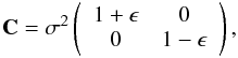 (17)with
the receiver specific parameters σ and ϵ reproduced in
Table 1.
(17)with
the receiver specific parameters σ and ϵ reproduced in
Table 1.
To simulate the optical system of the full Keck array, we drew 2480 realizations of beam size and ellipticity according to the receiver specifications and then used Eq. (16) to construct individual beams. We finally rotated the beams around their axes with randomly chosen angles between 0 ≤ φ < 2π. Applying fully random rotations is conservative since beams of bolometers in the same receiver are known to have similar orientations.
We found that only the first eight common eigenmodes are necessary to approximate all
2480 individual beams to a precision of at least the order
.
We illustrate this set of eigenmodes in Fig. 5. In
Fig. 6, we show as an example the beam with the
largest reconstruction error. For about 90 % of the detectors, the truncation errors are
below  .
.
We verified the results with a CMB simulation in flat sky approximation, high-pass filtered to suppress signal below ℓ < 50. We plot the difference map computed from a direct convolution and the compressed convolution with eight eigenmodes in Fig. 7. The error is subdominant on all angular scales.
The example outlined here demonstrates the full strength of the algorithm. Computing beam convolutions for the Keck array, we are able to reduce the number of computationally expensive convolution operations from 2480 to only eight, an improvement by a factor as high as 310.
Keck beam parameters as provided by Vieregg et al. (2012).
 |
Fig. 5 Simulated 2480 asymmetric Keck beams at 150 GHz are similar enough to be represented by only eight distinct beam eigenmodes to high precision. |
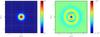 |
Fig. 6 Left panel: we show the beam with the largest
reconstruction error for the simulated Keck array. Right
panel: using the first eight beam eigenmodes, the truncation error is at
most of the order |
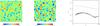 |
Fig. 7 Same as Fig. 4, but for the worst case of the simulated Keck experiment. Using eight beam modes for the convolution is sufficient to reduce the truncation error to negligible levels. |
4. Scope of the algorithm
As shown in Sect. 3, the algorithm has the potential to provide huge speedups for the beam convolution operation of modern experiments with a large number of detectors, necessary to improve the sensitivity of CMB measurements in the photon noise limited regime. Fast beam convolutions are not only important for the simulation of signal maps for individual detectors. They also play a crucial role in the mapmaking process, the iterative construction of a common sky map out of the time ordered data from different detectors observing at the same frequency.
Current experiments already deploy several hundreds to thousands of detectors, making them ideal candidates for the algorithm, e.g., SPTpol (about 800 pixels, Austermann et al. 2012), POLARBEAR (about 1300 pixels, Kermish et al. 2012), EBEX (about 1400 pixels, Reichborn-Kjennerud et al. 2010), Spider (about 2600 pixels, Filippini et al. 2010), ACTPol (about 3000 pixels, Niemack et al. 2010). For future experiments, the number of detectors can be expected to increase further, e.g., for PIPER (about 5000 pixels, Lazear et al. 2013), the Cosmic Origins Explorer (about 6000 pixels, The COrE Collaboration 2011), or POLARBEAR-2 (about 7500 pixels Tomaru et al. 2012), making the application of the algorithm even more rewarding.
The new method also allows a fast implementation of matched filtering on the sphere (or other domains) if the size of the target is unknown (e.g., to detect signatures of bubble collisions in the CMB, McEwen et al. 2012), or analogously for continuous wavelet transforms, frequently used in the context of data compression or pattern recognition (e.g., Mallat 1989). Here, the input signal is convolved with a large set of scale dilations of an analyzing filter or wavelet. Since the resulting convolution kernels are of similar shape by construction, the decomposition into only a few eigenmodes can be done efficiently. Our new method therefore has the potential to increase the numerical performance of such computations by a substantial factor.
Finally, besides from the reduction in computational costs, we note that compressed convolution may also offer the possibility to reduce the disk space required to store convolved data sets. Instead of saving the convolved signal for each kernel separately, it now becomes possible to just keep the compressed output for the most important eigenmodes, and efficiently decompress it with their proper weights for each individual kernel on the fly as needed.
5. Summary
In signal processing, a single data set often has to be convolved with many different kernels. With increasing data size, this operation quickly becomes numerically expensive to evaluate, possibly even dominating the execution time of analysis pipelines.
To increase the performance of such convolution operations, we introduced the general method of compressed convolution. Using an eigenvector decomposition of the convolution kernels, we first obtain their optimal expansion into a common set of basis functions. After ordering the modes according to their relative importance, we identify the minimal number of basis functions to retain to satisfy the accuracy requirements. Then, the convolution operation is executed for each mode separately, and the final result obtained for each kernel from a linear combination.
This algorithm offers particularly large performance improvements, if
-
the total number of kernels to consider is large, and
-
the kernels are sufficiently similar in shape, such that they can be approximated to good precision with only a few eigenmodes.
In case of the analysis of CMB data, we use the beam convolution problem as an example application of the compressed convolution scheme. On the basis of simulations of the Keck array with 2480 detectors (Vieregg et al. 2012), we demonstrated that the compressed convolution scheme allows to reduce the number of beam convolution operations by a factor of about 300, offering the possibility to cut the runtime of convolution pipelines by orders of magnitude. Additional improvements are possible when used in combination with efficient convolution algorithms (e.g., Elsner & Wandelt 2011).
If some eigenvalues do happen to be degenerate then the solutions will differ in ways that are not relevant to the compression efficiency.
Acknowledgments
The authors thank Clem Pryke for highlighting beam convolution for kilo-detector experiments as an outstanding problem, and Guillaume Faye and Xavier Siemens for conversations regarding the applications to searches for gravitational wave signals. B.D.W. was supported by the ANR Chaire d’Excellence and NSF grants AST 07-08849 and AST 09-08902 during this work. F.E. gratefully acknowledges funding by the CNRS. Some of the results in this paper have been derived using the HEALPix (Górski et al. 2005) package. Based on observations obtained with Planck (http://www.esa.int/Planck), an ESA science mission with instruments and contributions directly funded by ESA Member States, NASA, and Canada. The development of Planck has been supported by: ESA; CNES and CNRS/INSU-IN2P3-INP (France); ASI, CNR, and INAF (Italy); NASA and DoE (USA); STFC and UKSA (UK); CSIC, MICINN and JA (Spain); Tekes, AoF and CSC (Finland); DLR and MPG (Germany); CSA (Canada); DTU Space (Denmark); SER/SSO (Switzerland); RCN (Norway); SFI (Ireland); FCT/MCTES (Portugal); and PRACE (EU). A description of the Planck Collaboration and a list of its members, including the technical or scientific activities in which they have been involved, can be found at http://www.sciops.esa.int/index.php?project=planck&page=Planck_Collaboration.
References
- Austermann, J. E., Aird, K. A., Beall, J. A., et al. 2012, in Proc. SPIE, 8452, 1E [Google Scholar]
- Barreiro, R. B., & Hobson, M. P. 2001, MNRAS, 327, 813 [NASA ADS] [CrossRef] [Google Scholar]
- Cannon, K., Chapman, A., Hanna, C., et al. 2010, Phys. Rev. D, 82, 044025 [NASA ADS] [CrossRef] [Google Scholar]
- Cayón, L., Sanz, J. L., Barreiro, R. B., et al. 2000, MNRAS, 315, 757 [NASA ADS] [CrossRef] [Google Scholar]
- Elsner, F., & Wandelt, B. D. 2011, A&A, 532, A35 [NASA ADS] [CrossRef] [EDP Sciences] [Google Scholar]
- Elsner, F., & Wandelt, B. D. 2013, A&A, 549, A111 [NASA ADS] [CrossRef] [EDP Sciences] [Google Scholar]
- Filippini, J. P., Ade, P. A. R., Amiri, M., et al. 2010, in Proc. SPIE, 7741, 46 [Google Scholar]
- Górski, K. M., Hivon, E., Banday, A. J., et al. 2005, ApJ, 622, 759 [NASA ADS] [CrossRef] [Google Scholar]
- Jaranowski, P., & Królak, A. 2005, Liv. Rev. Relativity, 8, 3 [NASA ADS] [Google Scholar]
- Kermish, Z. D., Ade, P., Anthony, A., et al. 2012, in Proc. SPIE, 8452, 1C [Google Scholar]
- Lauer, T. 2002, in Proc. SPIE 4847, eds. J.-L. Starck, & F. D. Murtagh, 167 [Google Scholar]
- Lazear, J., Ade, P., Benford, D. J., et al. 2013, in American Astronomical Society Meeting Abstracts, 221, 229.04 [Google Scholar]
- Lupton, R., Gunn, J. E., Ivezić, Z., et al. 2001, in Astronomical Data Analysis Software and Systems X, eds. F. R. Harnden, Jr., F. A. Primini, & H. E. Payne, ASP Conf. Ser., 238, 269 [Google Scholar]
- Mallat, S. G. 1989, IEEE Trans. Pattern Anal. Mach. Intell., 11, 674 [Google Scholar]
- Martínez-González, E., Gallegos, J. E., Argüeso, F., Cayón, L., & Sanz, J. L. 2002, MNRAS, 336, 22 [NASA ADS] [CrossRef] [Google Scholar]
- McEwen, J. D., Hobson, M. P., Mortlock, D. J., & Lasenby, A. N. 2007, IEEE Trans. Signal Process., 55, 520 [NASA ADS] [CrossRef] [Google Scholar]
- McEwen, J. D., Feeney, S. M., Johnson, M. C., & Peiris, H. V. 2012, Phys. Rev. D, 85, 103502 [NASA ADS] [CrossRef] [Google Scholar]
- Natoli, P., de Gasperis, G., Gheller, C., & Vittorio, N. 2001, A&A, 372, 346 [NASA ADS] [CrossRef] [EDP Sciences] [Google Scholar]
- Niemack, M. D., Ade, P. A. R., Aguirre, J., et al. 2010, in Proc. SPIE, 7741, 51 [Google Scholar]
- Planck Collaboration 2011, A&A, 536, A1 [NASA ADS] [CrossRef] [EDP Sciences] [Google Scholar]
- Planck Collaboration 2014, A&A, in press [arXiv:1303.5068] [Google Scholar]
- Planck HFI Core Team 2011, A&A, 536, A4 [NASA ADS] [CrossRef] [EDP Sciences] [Google Scholar]
- Reichborn-Kjennerud, B., Aboobaker, A. M., Ade, P., et al. 2010, in Proc. SPIE, 7741, 37 [Google Scholar]
- Reinecke, M., & Seljebotn, D. S. 2013, A&A, 554, A112 [NASA ADS] [CrossRef] [EDP Sciences] [Google Scholar]
- Sheehy, C. D., Ade, P. A. R., Aikin, R. W., et al. 2010, in Proc. SPIE, 7741, 50 [Google Scholar]
- Tegmark, M. 1997, ApJ, 480, L87 [NASA ADS] [CrossRef] [Google Scholar]
- Tegmark, M., & de Oliveira-Costa, A. 1998, ApJ, 500, L83 [NASA ADS] [CrossRef] [Google Scholar]
- The COrE Collaboration 2011 [arXiv:1102.2181] [Google Scholar]
- Tomaru, T., Hazumi, M., Lee, A. T., et al. 2012, in Proc. SPIE, 8452, 1H [Google Scholar]
- Vieregg, A. G., Ade, P. A. R., Aikin, R., et al. 2012, in Proc. SPIE, 8452, 26 [Google Scholar]
- Wandelt, B. D., & Górski, K. M. 2001, Phys. Rev. D, 63, 123002 [NASA ADS] [CrossRef] [Google Scholar]
- Wiaux, Y., Jacques, L., Vielva, P., & Vandergheynst, P. 2006, ApJ, 652, 820 [NASA ADS] [CrossRef] [Google Scholar]
All Tables
All Figures
|
Fig. 1 All six Planck beams at 217 GHz (left panel) have very similar shapes. As a result, the eigenvalues of their singular value decomposition decrease quickly (right panel), allowing half of the modes to be safely discarded. |
| In the text | |
|
Fig. 2 Left panel: retaining the first three out of six
Planck 217 GHz beam eigenmodes allows to reduce the relative
truncation error of all convolution kernels to the order
|
| In the text | |
|
Fig. 3 Kernel weights allow for a full control over truncation errors. Same as Fig. 2, but for a
|
| In the text | |
|
Fig. 4 Truncation errors are negligible. Using the kernel with the largest truncation error as worst case scenario, we plot the beam convolved simulated CMB map used in this test of the Planck 217 GHz channels (left panel, we show a 10° × 10° patch). Middle panel: the difference map between the results obtained with the exact convolution and the compressed convolution with three beam modes. Right panel: compared to the fiducial power spectrum of the input map (dashed line), the power spectrum of the difference map is subdominant by a large margin on all angular scales. |
| In the text | |
|
Fig. 5 Simulated 2480 asymmetric Keck beams at 150 GHz are similar enough to be represented by only eight distinct beam eigenmodes to high precision. |
| In the text | |
|
Fig. 6 Left panel: we show the beam with the largest
reconstruction error for the simulated Keck array. Right
panel: using the first eight beam eigenmodes, the truncation error is at
most of the order |
| In the text | |
|
Fig. 7 Same as Fig. 4, but for the worst case of the simulated Keck experiment. Using eight beam modes for the convolution is sufficient to reduce the truncation error to negligible levels. |
| In the text | |
Current usage metrics show cumulative count of Article Views (full-text article views including HTML views, PDF and ePub downloads, according to the available data) and Abstracts Views on Vision4Press platform.
Data correspond to usage on the plateform after 2015. The current usage metrics is available 48-96 hours after online publication and is updated daily on week days.
Initial download of the metrics may take a while.