| Issue |
A&A
Volume 560, December 2013
|
|
|---|---|---|
| Article Number | A97 | |
| Number of page(s) | 8 | |
| Section | The Sun | |
| DOI | https://doi.org/10.1051/0004-6361/201322678 | |
| Published online | 11 December 2013 | |
Fast magnetoacoustic wave trains in magnetic funnels of the solar corona
1 Centre for Fusion, Space and Astrophysics, Department of
Physics, University of Warwick, CV4 7AL, UK
e-mail:
This email address is being protected from spambots. You need JavaScript enabled to view it.
2
School of Space Research, Kyung Hee University,
Yongin,
446-701
Gyeonggi,
Korea
3
Central Astronomical Observatory at Pulkovo of the Russian Academy
of Sciences, 196140
St Petersburg,
Russia
Received:
16
September
2013
Accepted:
28
October
2013
Abstract
Context. Fast magneto-acoustic waves are highly dispersive in waveguides, so they can generate quasi-periodic wave trains if a localised, impulsive driver is applied. Such wave trains have been observed in the solar corona and may be of use as a seismological tool since they depend upon the plasma structuring perpendicular to the direction of propagation.
Aims. We extend existing models of magnetoacoustic waveguides to consider the effects of an expanding magnetic field. The funnel geometry employed includes a field-aligned density structure.
Methods. We performed 2D numerical simulations of impulsively generated fast magneto-acoustic perturbations. The effects of the density contrast ratio, density stratification, and spectral profile of the driver upon the excited wave trains were investigated.
Results. The density structure acts as a dispersive waveguide for fast magneto-acoustic waves and generates a quasi-periodic wave train similar to previous models. The funnel geometry leads to generating additional wave trains that propagate outside the density structure. These newly discovered wave trains are formed by the leakage of transverse perturbations, but they propagate upwards owing to the refraction caused by the magnetic funnel.
Conclusions. The results of our funnel model may be applicable to wave trains observed propagating in the solar corona. They demonstrate similar properties to those found in our simulations.
Key words: magnetohydrodynamics (MHD) / Sun: atmosphere / Sun: corona / Sun: magnetic fields / Sun: oscillations / waves
© ESO, 2013
1. Introduction
Fast magnetoacoustic waves are easily guided by plasma non-uniformities stretched along the magnetic field (see, e.g. Van Doorsselaere et al. 2008). The guided waves, also called “modes” of the waveguiding plasma structures, are dispersive; i.e., their phase and group speeds depend on the frequency and the wavelength. This kind of dispersion is known as geometrical, since it is prescribed by the presence of a characteristic spatial scale in the system, the width of the waveguiding non-uniformity (Roberts et al. 1983, 1984). More specifically, in the low-β plasma of coronal active regions, the phase speed of all fast magneto-acoustic modes decreases with the decrease in the wavelength. Fast waves of longer periods propagate at higher phase speeds. Waves of all azimuthal symmetry: sausage (m = 0), kink (m = 1), and fluting (m > 1), where m is the integer azimuthal wave number, have this property. The dependence of the group speed on the period is more complicated. If the profile of the plasma non-uniformity is steep enough, it has a minimum at a certain wavelength (Nakariakov & Roberts 1995). This dispersive feature motivated Roberts et al. (1984) to propose that a development of a broadband initial excitation in a fast magneto-acoustic waveguide would result in the formation of a quasi-periodic fast wave train. Indeed, as different spectral components propagate at different speeds, they arrive at a sufficiently remote observational point at different instants of time. Moreover, Roberts et al. (1984) have argued that the typical characteristic signature of such a wave train would have three distinct phases. This result was consistent with the variations in the radio emission observed in solar flares (Roberts et al. 1983). This first encouraging result stimulated a number of follow-up theoretical and observational studies.
In the series of early numerical experiments on the initial stage of the dispersive evolution of guided fast wave trains confirmed the formation of a quasi-periodic wave pattern in both linear (Murawski & Roberts 1993a,b, 1994) and nonlinear (Murawski & Roberts 1993c,d) regimes. More advanced numerical simulations of the developed stage of the evolution have shown that a more adequate description of the formed quasi-periodic wave pattern could be obtained with the use of wavelet analysis (Nakariakov et al. 2004). It was shown that a very robust feature of such a wave train is the “crazy tadpole” wavelet spectrum, with a quasi-monochromatic low-amplitude, low-frequency “tail” preceding the relatively broad-band, shorter-frequency larger amplitude “head”. Moreover, this observational feature was found in the propagating fast wave trains detected with the Solar Eclipse Coronal Imaging System (SECIS) (Katsiyannis et al. 2003; Cooper et al. 2003). Development of that study revealed that, for the perturbations of the sausage symmetry, an important factor is also the broadness of the initial spectrum in comparison with the cut-off wavelength (Nakariakov et al. 2005) and that in some cases the wavelet spectrum of the resulting wave train could be almost monochromatic.
Similar tadpole wavelet features were detected in a number of flare-associated radio bursts observed in the decimetric band (Mészárosová et al. 2009a,b,a, 2011; Karlický et al. 2011; Mészárosová et al. 2013). In particular, observations with the spatial resolution revealed the appearance of signals with the tadpole wavelet signatures in a fan structure above a coronal magnetic null point (Mészárosová et al. 2013). Recently, fibre-burst spectral features observed in the radio band were interpreted in terms of propagating fast sausage magneto-acoustic wave trains (Karlický et al. 2013). Detailed numerical studies have demonstrated the formation of very characteristic wave trains also in current sheets (Jelínek & Karlický 2012). This effect was found to be robust, and was confirmed to occur in vertical, gravitationally stratified current sheets typical of the standard model of a solar flare (Jelínek et al. 2012; Karlický et al. 2013).
High time resolution and sensitivity of the Solar Dynamics Observatory/Atmospheric Imaging Assembly (AIA) instrument allowed for detection of propagating fast wave trains in the extreme UV (EUV) band. Liu et al. (2011) detected disturbances of EUV emission that emanated near the flare kernel and propagated outwards up to about 400 Mm along a funnel of coronal loops at the phase velocity of about 2000 km s-1, with the main period of about 3 min. Ofman et al. (2011) interprets these propagating disturbances as fast magnetoacoustic waves driven quasi-periodically at the base of the flaring region. The model included the dipole magnetic field and gravitationally stratified density at coronal temperature. At the coronal base, the fast magneto-acoustic wave was excited by periodic velocity pulsations in the horizontal plane confined to a funnel of magnetic field lines, associated with quasi-periodic energy releases with the same 3-min period. Similar fast waves were seen in several other events. In particular, Shen & Liu (2012) observed fast waves of the EUV intensity with several periodicities ranging from 25 s to 134 s. The periodicity was linked with quasi-periodic variations of the soft X-ray intensity in the solar flare that was believed to be the driver of the waves. Liu et al. (2012) detected fast waves with the dominating periodicity of 2 min, also associated with quasi-periodic pulsations in the accompanying flare. However, there was also another class of observed waves with the shorter periods of about 47 s.
In a uniform medium, fast magnetoacoustic waves do not propagate along the magnetic field. But, because the fast waves are observed to propagate along the magnetic field, they should be guided by transverse structuring of the fast speed: locally the waves are oblique and travel along the field because of refraction or reflection (e.g. Van Doorsselaere et al. 2008). If the fast waves are generated by impulsive energy releases and guided by plasma non-uniformities, they should be subject to dispersive evolution. In this paper, we aim to study the effect of dispersive evolution on magnetic funnels of the solar corona.
2. Model setup
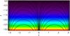 |
Fig. 1 Magnetic field lines for our equilibrium. The magnetic field describes an expanding funnel at the centre of the numerical domain. The contour represents the magnitude of the magnetic field, which varies exponentially with height. |
In this work we restrict ourselves to a simple 2D equilibrium that allows us to emphasise
the main features of the wave propagation and perform a controlled parametric study. The
equilibrium magnetic configuration is a potential magnetic field 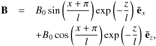 (1)where
B0 and l are constant, controlling the size
of the field and the characteristic spatial scale, respectively. In the following, we
consider x and z as the horizontal and vertical
coordinates, respectively. Using the components of the field vector given by Eq. (1), one can readily obtain the equation of the
field lines,
(1)where
B0 and l are constant, controlling the size
of the field and the characteristic spatial scale, respectively. In the following, we
consider x and z as the horizontal and vertical
coordinates, respectively. Using the components of the field vector given by Eq. (1), one can readily obtain the equation of the
field lines,  (2)where
C is a constant determining the individual field lines. Figure 1 shows the geometry of the field. The absolute value of
the field is
(2)where
C is a constant determining the individual field lines. Figure 1 shows the geometry of the field. The absolute value of
the field is  (3)thus it is constant in
the horizontal direction, as demonstrated by the contour plot of Fig. 1. Since our equilibrium is strongly related to trigonometric functions
and it is convenient for us to consider a domain of width 2π, we continue
to use dimensionless units throughout this paper. Results may be converted to physical units
by choosing appropriate normalisation constants; e.g., dimensionless length scales
(
(3)thus it is constant in
the horizontal direction, as demonstrated by the contour plot of Fig. 1. Since our equilibrium is strongly related to trigonometric functions
and it is convenient for us to consider a domain of width 2π, we continue
to use dimensionless units throughout this paper. Results may be converted to physical units
by choosing appropriate normalisation constants; e.g., dimensionless length scales
( ),
time scales (
),
time scales ( ),
and speeds (
),
and speeds ( )
can be converted to physical ones (x, t, and
v) using
)
can be converted to physical ones (x, t, and
v) using  ,
,
 , and
, and
 , where
l0, t0, and
v0 are the chosen normalisation constants for length scales,
times, and speeds, respectively, and
v0 = l0/t0
(see example in Sect. 4).
, where
l0, t0, and
v0 are the chosen normalisation constants for length scales,
times, and speeds, respectively, and
v0 = l0/t0
(see example in Sect. 4).
The equilibrium plasma density is taken as a modified symmetric Epstein profile. At each
horizontal level, the density in the funnel is given by an Epstein profile (see, e.g. Nakariakov & Roberts 1995; Pascoe et al. 2007), with the characteristic width of the profile growing
with height such that the profile remains aligned with the magnetic field lines. Also, the
density is taken to be hydrostatically stratified, with the effective scale height
Λeff. The value of Λeff = Λcos α is greater than
the density scale height Λ ≈ 50T, where T is the plasma
temperature measured in MK, the scale height is measured in Mm, and α is
the angle of the funnel axis from the vertical direction. Thus, the equilibrium density is
given by the expression ![Mathematical equation: \begin{eqnarray} \rho_0 &= & \, \exp\left( -\frac{z + \pi}{\Lambda_\mathrm{eff}} \right) \notag\\ && \times \left[ \left( \rho_\mathrm{F} - \rho_\infty \right) \mathrm{sech}^2 \left( \frac{x/l}{\arccos \exp (z/l) -\pi/2} \right)^{p} + \rho_\infty, \right] \label{rho} \end{eqnarray}](/articles/aa/full_html/2013/12/aa22678-13/aa22678-13-eq33.png) (4)where
ρ∞ is the density far from the funnel, taken as constant for
simplicity, and ρF is the departure of the density in the centre
of the funnel at the height z = −π from the background
density ρ∞. The value of ρF can be
either positive or negative, with
| ρF| < ρ∞.
The index p allows one to control the steepness of the transverse profile
of the density. The internal density ρF can be either greater or
lower than the external density ρ∞. For p → ∞
the profile degenerates into a step function. Figure 2
shows the density profile for a funnel with density contrast
ρF/ρ∞ = 3,
p = 8, l = 1, and we first consider the case of no
density stratification Λeff → ∞. Figure 3
shows the dependence of the half width a of the funnel upon height
z. The funnel has a ≈ 0.1 at the location of the initial
perturbation (z = −3π/4), and
a ≈ 0.2 at
z = −π/2 where wave train signals
will be measured (see Sect. 3).
(4)where
ρ∞ is the density far from the funnel, taken as constant for
simplicity, and ρF is the departure of the density in the centre
of the funnel at the height z = −π from the background
density ρ∞. The value of ρF can be
either positive or negative, with
| ρF| < ρ∞.
The index p allows one to control the steepness of the transverse profile
of the density. The internal density ρF can be either greater or
lower than the external density ρ∞. For p → ∞
the profile degenerates into a step function. Figure 2
shows the density profile for a funnel with density contrast
ρF/ρ∞ = 3,
p = 8, l = 1, and we first consider the case of no
density stratification Λeff → ∞. Figure 3
shows the dependence of the half width a of the funnel upon height
z. The funnel has a ≈ 0.1 at the location of the initial
perturbation (z = −3π/4), and
a ≈ 0.2 at
z = −π/2 where wave train signals
will be measured (see Sect. 3).
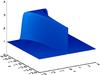 |
Fig. 2 Density profile for a funnel with density contrast ρF/ρ∞ = 3, p = 8, and no stratification Λeff → ∞. The profile follows the magnetic field lines of Fig. 1. |
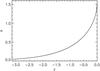 |
Fig. 3 Dependence of the half width a of the funnel upon height z for the equilibrium shown in Figs. 1 and 2. |
 |
Fig. 4 Dependence of the phase (top) and group (bottom) speeds on the normalised wave number ka for the transverse density profile used in Fig. 2. The upper and lower dashed lines represent the external and internal Alfvén speeds, respectively. |
Figure 4 shows the “local” dispersion curves for trapped sausage perturbations of the transverse density profile used in Eq. (4) and Fig. 2 at a certain fixed height z. The phase (top) and group (bottom) speeds are shown as a function of the wave number k = 2π/λ normalised to the half width of the density profile a (see Fig. 3). The upper and lower dashed lines represent the external and internal Alfvén speeds, respectively. The excitation of oscillations over a range of wave numbers by a localised, impulsive perturbation results in two kinds of wave motions: trapped modes guided along the axis of the funnel and leaky waves going away from the funnel. The trapped modes appear from the spectral energy with the wave numbers greater than the cut-off value that corresponds to the phase speed being equal to the external Alfvén speed (the leftmost value of the dispersive curve in Fig. 4). The leaky waves are excited by the part of the spectrum with the wave numbers smaller than the cut-off value. In contrast to the trapped waves that are confined to the waveguiding plasma non-uniformity, leaky waves propagate away from the waveguiding non-uniformity (Cally 1986; Nakariakov et al. 2012). In this case the non-uniformity acts as a fast magneto-acoustic antenna. Physically, the difference between trapped and leaky components is determined by the local incidence angle of the wave to the boundary of the non-uniformity in comparison with the angle of total internal reflection. The spectral components with longitudinal wave numbers smaller than the cut-off value, hence with an incidence angle closer to normal than the total internal reflection angle, become leaky: a part of their energy escapes to the external medium during each act of reflection. Propagation of these different spectral components of the guided modes at different speeds leads to formation of a quasi-periodic wave train (Nakariakov et al. 2004). The particular signal measured depends upon the details of the driver, the waveguide, and the distance of the point of measurement from the initial perturbation (Nakariakov et al. 2005). The group speed possesses a minimum, which is the case for all p > 1 (Nakariakov & Roberts 1995), and the chosen density profile steepness of p = 8 is large enough that the results differ from those of the step profile (p → ∞) by only ~1%. On the other hand, the profile is smooth enough to be resolved well in our simulations (e.g. Fig. 2), so we avoid introducing discontinuities.
The applied density structure is defined to be in equilibrium by defining the internal
energy density as 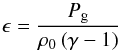 (5)where
Pg is a constant gas pressure and
γ = 5/3 is the ratio of specific heat capacities.
Since the magnetic field strength decreases as a function of height z and
the gas pressure is constant, plasma β increases with height. We choose to
consider a low β plasma, with
β < 6 × 10⁻⁴ throughout the numerical
domain.
(5)where
Pg is a constant gas pressure and
γ = 5/3 is the ratio of specific heat capacities.
Since the magnetic field strength decreases as a function of height z and
the gas pressure is constant, plasma β increases with height. We choose to
consider a low β plasma, with
β < 6 × 10⁻⁴ throughout the numerical
domain.
The equilibrium given by Eqs. (1), (4), (5) is perturbed in the transverse direction by a spatially localised function
![Mathematical equation: \begin{equation} V_x = A \frac{x}{l} \exp \left[ - \left(\frac{x/l}{\Delta_x}\right)^2\right] \exp \left[ - \left(\frac{z/l+3\pi/4}{\Delta_z}\right)^2\right], \label{saus_pert} \end{equation}](/articles/aa/full_html/2013/12/aa22678-13/aa22678-13-eq58.png) (6)where A is
the initial amplitude, taken to be small enough to avoid nonlinear effects, and the
parameters Δx and Δz are the width
of the initial pulse in the horizontal and vertical directions, respectively. Expression
(6) is an odd function with respect to the
horizontal coordinate x, so it describes the excitation of sausage
perturbations. We begin by considering Δx = 0.05 and
Δz = 0.05. This choice of Δx
sets the width of the initial excitation to be similar to the width of the funnel at this
height. The effect of varying Δz is considered in Sect. 3.1.
(6)where A is
the initial amplitude, taken to be small enough to avoid nonlinear effects, and the
parameters Δx and Δz are the width
of the initial pulse in the horizontal and vertical directions, respectively. Expression
(6) is an odd function with respect to the
horizontal coordinate x, so it describes the excitation of sausage
perturbations. We begin by considering Δx = 0.05 and
Δz = 0.05. This choice of Δx
sets the width of the initial excitation to be similar to the width of the funnel at this
height. The effect of varying Δz is considered in Sect. 3.1.
Our typical resolution is 4000 × 2000 grid points for a numerical domain of size 2π × π. The results of a convergence test at a resolution of 8000 × 4000 grid points produced results that differed by less than 0.2%. Line-tied boundary conditions were used, with damping layers near the edges of the numerical domain to avoid perturbations reflecting back inwards. Simulations were preformed using the 2.5D MHD code Lare2d (Arber et al. 2001), which operates by taking a Lagrangian predictor-corrector time step, after which variables are conservatively remapped back onto the original Eulerian grid using van Leer gradient limiters. The governing equations simulated by the code are the (normalised) ideal MHD equations with an adiabatic equation of state. In our simulations, the 2.5D approximation corresponds to having no variations in the y-direction i.e. ∂/∂y = 0.
3. Results
The fast wave train is generated by applying a perturbation given by Eq. (6) near the bottom of the numerical domain. The density enhancement (Eq. (4)) defines a local minimum in the Alfvén speed, so it acts as a waveguide for the fast sausage perturbations. Wave trains propagate upwards and downwards along the density structure. We focus on the behaviour of the upwards-propagating wave trains. The downwards-propagating waves are also damped as they approach the lower boundary. Since the plasma β is very small but finite and our perturbation compressive, we also generate a slow wave, but this propagates an insignificant distance during our simulation, so we are not concerned with its behaviour in this paper.
The transverse size of the perturbation Δx was chosen to be similar to the transverse size of the funnel where the perturbation is applied. The generated fast sausage wave train therefore undergoes dispersive evolution, similar to previous studies, owing to the presence of this characteristic transverse length scale provided by the waveguide. However, as the wave train propagates to higher z, the density structure expands as the funnel follows the magnetic field lines (Eq. (1)). This increase in the characteristic transverse length scale leads to the wave train undergoing less dispersive evolution as it propagates. (In the limit of a → ∞, the medium is uniform and dispersionless.)
In the other limit, as ka → 0, we must take another property of sausage modes into account; the existence of a cut-off wave number which leads to leakage. The effect of the cut-off wave number in the case of a uniform slab is discussed in Sect. 2. Likewise, in the case of a funnel, for an initial perturbation with a sufficiently large longitudinal extent, some fraction of the spatial spectrum of the perturbation will correspond to wavelengths that are longer than the cut-off wavelength. Perturbations with larger longitudinal scales have narrower spatial spectra and so more of the energy is localised at wave numbers smaller than the cut-off wave number (Nakariakov et al. 2005).
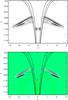 |
Fig. 5 Snapshot of velocity | v | (top) and density
(bottom) perturbations at |
For our applied perturbation, we therefore have a component of the wave train that falls below the sausage mode cut-off and leaks out of the waveguide. The wavelength of the longest trapped component of the wave train depends upon the density contrast ratio and the width of the waveguide. For our chosen density structure in this paper, the density contrast remains constant with height. The increase in the width of the waveguide with height suggests that the funnel becomes less leaky with height. The components of the wave train that are trapped and propagate along the axis of the waveguide continue to remain trapped at greater heights. Most of the leakage therefore occurs at the start of the simulation when the wave trains are generated.
Just after the initial perturbation, we therefore have the separation of the fast sausage wave train into two distinct parts: the trapped part that propagates along the waveguide axis, and the leaky part that propagates away from the waveguide. In previous work (e.g. Pascoe et al. 2007) when a straight waveguide is considered, the leaky components propagate perpendicular to the waveguide and out of the system. In our current model, however, the magnetic field strength varies as a function of height as given by Eq. (3). The wave train propagation speed therefore decreases with increasing z, so the leaky wave train undergoes refraction and also propagates upwards in our model. These leaky wave trains are generated both to the left and right of the funnel, so we denote them as “wing” wave trains to distinguish them from the usual wave train that propagates along the waveguide.
A snapshot of simulation variables at  is shown in Fig. 5. The upper panel shows the perturbations in the absolute
value of the velocity, with the line contours outlining the boundary of the density profile.
The trapped wave train can be seen within the funnel density structure at
z ≈ −1, while the wing wave trains are outside and on either side of the
density structure, and they have propagated further in the z-direction.
Within the funnel the wave train is formed by perturbations to the transverse velocity
vx, and perturbations vanish along the funnel
axis, in accordance with the anti-symmetric nature of the sausage-mode transverse velocity
profile. The bottom panel of Fig. 5 shows the
corresponding density perturbations. For the trapped wave train, these are greatest along
the funnel axis, where the sausage mode velocity has a node. In comparison, the wing wave
train mainly comprises vertical velocity perturbations
vz, propagating in phase with density
perturbations. Consistent with fast wave behaviour, the wave fronts propagate both across
and along (in the guided regime) field lines. The wave front may continue to expand, though
in these simulations it is restricted by the boundaries of the numerical domain (and the
damping layers located there). For clarity in Fig. 5
the numerical domain has been cropped to focus on the wave trains. The horizontal and
vertical scales are unequal, which exaggerates the propagation angle of the wing wavefront,
which is around ten degrees from vertical by this stage.
is shown in Fig. 5. The upper panel shows the perturbations in the absolute
value of the velocity, with the line contours outlining the boundary of the density profile.
The trapped wave train can be seen within the funnel density structure at
z ≈ −1, while the wing wave trains are outside and on either side of the
density structure, and they have propagated further in the z-direction.
Within the funnel the wave train is formed by perturbations to the transverse velocity
vx, and perturbations vanish along the funnel
axis, in accordance with the anti-symmetric nature of the sausage-mode transverse velocity
profile. The bottom panel of Fig. 5 shows the
corresponding density perturbations. For the trapped wave train, these are greatest along
the funnel axis, where the sausage mode velocity has a node. In comparison, the wing wave
train mainly comprises vertical velocity perturbations
vz, propagating in phase with density
perturbations. Consistent with fast wave behaviour, the wave fronts propagate both across
and along (in the guided regime) field lines. The wave front may continue to expand, though
in these simulations it is restricted by the boundaries of the numerical domain (and the
damping layers located there). For clarity in Fig. 5
the numerical domain has been cropped to focus on the wave trains. The horizontal and
vertical scales are unequal, which exaggerates the propagation angle of the wing wavefront,
which is around ten degrees from vertical by this stage.
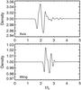 |
Fig. 6 Density signals measured inside (top) and outside (bottom) the funnel density structure. |
Figure 6 shows the density perturbation signals as a function of time measured at two points: one along the funnel axis x = 0, and the other outside the funnel at x = −π/2, where the wing wave train passes. The signals are taken at the same height of z = −π/2 (with the initial perturbation at z = −3π/4). Figure 7 shows the wavelets corresponding to the signals in Fig. 6. Both the trapped and the wing wave trains are quasi-periodic. The perturbations are much smaller than the equilibrium density values (here, 3 at the funnel axis and 1 far from the axis), in accordance with the small amplitude used in Eq. (6). Since the wing wave trains are formed from the leaky components of the initial perturbation, it typically comprises periods that are longer than the trapped wave train. However, in Fig. 7, the wavelet spectrum for the wing wave train shows it is in fact composed of comparable (and even shorter) periods than the one in the waveguide. This discrepancy can be understood as due to the variation in the magnetic field strength and Alfvén speed, with a height that causes the wavelengths of the wave trains to shorten as they propagate upwards.
In Fig. 7 (and later wavelet figures) the colour panel represents the wavelet (Morlet) power spectrum of the signal. The four colour contours correspond to levels of wavelet power higher than 0.2, 0.4, 0.6, and 0.8 times the maximum value. The solid contour shows the 99% significance level, estimated according to Torrence & Compo (1998). To aid visualisation, the normalised time profile of the signal is superimposed on the wavelet spectrum as a thick solid line. The cross-hatched regions on either end of the wavelet spectrum indicate the cone of influence. The panel on the right of the wavelet spectrum represents the global wavelet power spectrum (WPS) of the signal. The dashed line on this plot defines the 99% significance level.
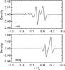 |
Fig. 8 Spatial cuts for the axis (top) and wing (bottom). |
Figure 8 shows the spatial profile of the trapped and
wing wave trains at . By this time, the wing wave
train has propagated higher than the trapped wave train due to the external Alfvén speed
being larger than the internal Alfvén speed (and both decreasing with height in accordance
with Eq. (3)). The wavelet spectra shown in
Fig. 9 demonstrate that the signals at this time have
similar wavelengths λ ~ 0.1.
Figure 10 shows the wing wave train plotted at times
, 2.5, and 1.75. As the wave train
propagates upwards, the Alfvén speed decreases, so the wavelengths of the quasi-periodic
signal decrease. The amplitude of the perturbations increases with distance travelled.
Figure 11 shows the evolution of the trapped wave
train as it propagates. In the top panel, the signals at times
and 2.5 are normalised to a
common maximum and shifted in height to lie on top of each other. The wavelet spectra for
and
 are shown in the middle and
bottom panels, respectively, and demonstrate the decrease in wavelength at the later time.
Figure 12 shows the same analysis for the wing wave
train, for which the shift in wavelengths is greater, in accordance with the larger
(vertical) distance travelled due to the higher Alfvén speed.
are shown in the middle and
bottom panels, respectively, and demonstrate the decrease in wavelength at the later time.
Figure 12 shows the same analysis for the wing wave
train, for which the shift in wavelengths is greater, in accordance with the larger
(vertical) distance travelled due to the higher Alfvén speed.
3.1. Effect of driver profile on “wing” wave train
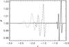 |
Fig. 10 Evolution of wing wave train with distance. The signal is plotted at times
|
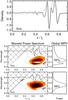 |
Fig. 11 Evolution of the trapped wave train. The signals at times
|
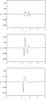 |
Fig. 13 Wing density signals for Δz of 0.02 (top), 0.1 (middle), and 0.5 (bottom). |
Nakariakov et al. (2005) demonstrates how the spectral profile of the wave trains depends upon the longitidunal wavelength of the initial pulse. Pulses with larger longitudinal sizes Δz are composed of a narrower range of wave numbers and so produce wave trains that are more monochromatic. In Fig. 13 we show the wing signals generated by pulses with different values of Δz. For higher values of Δz, the signal becomes less quasi-periodic and appears more like a single pulse, consistent with the more monochromatic spatial spectra of their source.
3.2. Density contrast ratio
 |
Fig. 14 Density profile for a funnel with density contrast ρF/ρ∞ = 10, p = 8, and no stratification. |
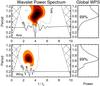 |
Fig. 15 Density signals and wavelets measured inside (top) and outside (bottom) the funnel density structure for ρF/ρ∞ = 10. |
Figure 14 shows the density profile for a funnel with a higher density contrast ratio of ρF/ρ∞ = 10, with all other parameters remaining the same as in previous sections. For higher density contrasts, the difference between the internal and external Alfvén speeds increases, and so a wider range of periodicities is supported by the structure. Figure 15 shows the wavelet signatures for the simulation with the higher density. The typical periods in the wave trains are longer in comparison with the lower density simulation (Fig. 7).
3.3. Effect of stratification
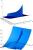 |
Fig. 16 Density (top) and Alfvén speed (bottom) profiles for a funnel with density contrast ρF/ρ∞ = 3, p = 8 and stratification with Λeff = 2. The background density has the same vertical stratification, such that the density contrast ratio remains constant with height. |
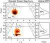 |
Fig. 17 Density signals and wavelets measured inside (top) and outside (bottom) the stratified funnel shown in Fig. 16. |
Next we consider the effect of vertical density stratification, which is determined in our equilibrium by the parameter Λeff. Figure 16 shows the density profile for a funnel with Λeff = 0.02, with the external medium also having the same vertical stratification such that the density contrast ratio remains constant with height. The density signals and their wavelets for this structure are shown in Fig. 17. By comparing to Fig. 7 we see that the density stratification does not dramatically alter the wave trains, though there is a shift in wavelet power to smaller periodicities. The effect of the magnetic geometry (with intrinsic magnetic stratification) is the dominant feature of the funnel.
4. Discussion
In this paper we have presented the first results of studying the behaviour of impulsively generated fast magnetoacoustic waves in a funnel geometry. The funnel comprises a density enhancement that is field-aligned and that expands with height. This structure acts as a waveguide, so when we apply our compressive driver we generate fast sausage waves that propagate along the funnel. Their dispersive nature leads to the formation of a quasi-periodic wave train, similar to wave trains generated in previously considered geometries such as straight slabs and cylinders.
Owing to the existence of a cut-off wave number for the sausage mode and to the localised nature of our driver, some of the fast wave energy leaks out of the waveguide. In our funnel model, these waves undergo refraction due to the variation in the magnetic field strength with height, so they also propagate upwards. We therefore obtain the result of quasi-periodic “wing” fast magnetoacoustic wave trains propagating outside of the funnel density structure, but having properties that depend upon the details of the structure and the driver.
The existence of these additional wave trains might account for certain wave behaviour observed in the solar corona after impulsive energy release, such as flares. Yuan et al. (2013) report the observation of a series of quasi-periodic propagating fast wave trains associated with bursts in radio emission due to flaring energy releases. The wave front was resolved using SDO/AIA and was seen to expand as the wave train propagates. Measurements of the amplitude of the wave trains reveal that it increased and then decreased again. This may be understood in terms of competition between amplification of the wave due to stratification as it propagates, and attenuation of the wave front due to expansion.
These properties are consistent with the features of the wing wave trains we obtain in our simulations. Figure 10 shows the increase in the amplitude of the wave train as it propagates upwards in the magnetically stratified medium, similar to the open corona. Our simulations are performed in a 2D geometry so the expansion of the wave front that causes the decay of the amplitude is likely to be more pronounced in 3D. The wave fronts are observed in AIA intensity perturbations that are in-phase perpendicular to the direction of travel, similar to the perturbations shown in Fig. 5. The observed wave trains were also seen to decelerate, again consistent with our model.
If we consider the wave trains observed by Yuan et al.
(2013) in more detail, they report (for Train-2) a period of 40 ± 0.5 s,
λ = 24.4 ± 0.1 Mm, and so a corresponding phase speed
ω/k = λ/P = 0.61
Mm/s. If we consider the numerical simulations presented in Figs. 6−9, we have (in dimensionless units)
 and
and
 , with
 . We may therefore compare our
numerical results to the observations of Yuan et al.
(2013) by choosing normalisation constants l0 = 200 Mm
and v0 = 2 Mm/s, which give P ≈ 40 s,
λ ≈ 24 Mm, and
ω/k ≈ 0.6 Mm/s. This choice of
normalisation also implies that the wave train in our simulation would have travelled ≈150
Mm, which is consistent with Fig. 1c of Yuan et al.
(2013), and the funnel would have a half width a ≈ 20 Mm near the
point of excitation.
. We may therefore compare our
numerical results to the observations of Yuan et al.
(2013) by choosing normalisation constants l0 = 200 Mm
and v0 = 2 Mm/s, which give P ≈ 40 s,
λ ≈ 24 Mm, and
ω/k ≈ 0.6 Mm/s. This choice of
normalisation also implies that the wave train in our simulation would have travelled ≈150
Mm, which is consistent with Fig. 1c of Yuan et al.
(2013), and the funnel would have a half width a ≈ 20 Mm near the
point of excitation.
Acknowledgments
This work is supported by the Marie Curie PIRSES-GA-2011-295272 RadioSun project, the European Research Council under the SeismoSun Research Project No. 321141 (DJP, VMN), grant 8524 of the Ministry of Education and Science of the Russian Federation (VMN), a Kyung Hee University International Scholarship (VMN), and the Russian Foundation of Basic Research under grant 13-02-00044. The computational work for this paper was carried out on the joint STFC and SFC (SRIF) funded cluster at the University of St Andrews (Scotland, UK). Wavelet software was provided by C. Torrence and G. Compo, and is available at URL: http://atoc.colorado.edu/research/wavelets/.
References
- Arber, T., Longbottom, A., Gerrard, C., & Milne, A. 2001, J. Comput. Phys., 171, 151 [NASA ADS] [CrossRef] [Google Scholar]
- Cally, P. S. 1986, Sol. Phys., 103, 277 [NASA ADS] [CrossRef] [Google Scholar]
- Cooper, F. C., Nakariakov, V. M., & Williams, D. R. 2003, A&A, 409, 325 [NASA ADS] [CrossRef] [EDP Sciences] [Google Scholar]
- Jelínek, P., & Karlický, M. 2012, A&A, 537, A46 [NASA ADS] [CrossRef] [EDP Sciences] [Google Scholar]
- Jelínek, P., Karlický, M., & Murawski, K. 2012, A&A, 546, A49 [NASA ADS] [CrossRef] [EDP Sciences] [Google Scholar]
- Karlický, M., Jelínek, P., & Mészárosová, H. 2011, A&A, 529, A96 [NASA ADS] [CrossRef] [EDP Sciences] [Google Scholar]
- Karlický, M., Mészárosová, H., & Jelínek, P. 2013, A&A, 550, A1 [NASA ADS] [CrossRef] [EDP Sciences] [Google Scholar]
- Katsiyannis, A. C., Williams, D. R., McAteer, R. T. J., et al. 2003, A&A, 406, 709 [NASA ADS] [CrossRef] [EDP Sciences] [Google Scholar]
- Liu, W., Title, A. M., Zhao, J., et al. 2011, ApJ, 736, L13 [NASA ADS] [CrossRef] [Google Scholar]
- Liu, W., Ofman, L., Nitta, N. V., et al. 2012, ApJ, 753, 52 [NASA ADS] [CrossRef] [Google Scholar]
- Mészárosová, H., Karlický, M., Rybák, J., & Jiřička, K. 2009a, ApJ, 697, L108 [NASA ADS] [CrossRef] [Google Scholar]
- Mészárosová, H., Sawant, H. S., Cecatto, J. R., et al. 2009b, Adv. Space Res., 43, 1479 [NASA ADS] [CrossRef] [Google Scholar]
- Mészárosová, H., Karlický, M., & Rybák, J. 2011, Sol. Phys., 273, 393 [NASA ADS] [CrossRef] [Google Scholar]
- Mészárosová, H., Dudík, J., Karlický, M., Madsen, F. R. H., & Sawant, H. S. 2013, Sol. Phys., 283, 473 [NASA ADS] [CrossRef] [Google Scholar]
- Murawski, K., & Roberts, B. 1993a, Sol. Phys., 143, 89 [NASA ADS] [CrossRef] [Google Scholar]
- Murawski, K., & Roberts, B. 1993b, Sol. Phys., 144, 101 [NASA ADS] [CrossRef] [Google Scholar]
- Murawski, K., & Roberts, B. 1993c, Sol. Phys., 144, 255 [NASA ADS] [CrossRef] [Google Scholar]
- Murawski, K., & Roberts, B. 1993d, Sol. Phys., 145, 65 [Google Scholar]
- Murawski, K., & Roberts, B. 1994, Sol. Phys., 151, 305 [NASA ADS] [CrossRef] [Google Scholar]
- Nakariakov, V. M., & Roberts, B. 1995, Sol. Phys., 159, 399 [NASA ADS] [CrossRef] [Google Scholar]
- Nakariakov, V. M., Arber, T. D., Ault, C. E., et al. 2004, MNRAS, 349, 705 [NASA ADS] [CrossRef] [Google Scholar]
- Nakariakov, V. M., Pascoe, D. J., & Arber, T. D. 2005, Space Sci. Rev., 121, 115 [NASA ADS] [CrossRef] [Google Scholar]
- Nakariakov, V. M., Hornsey, C., & Melnikov, V. F. 2012, ApJ, 761, 134 [NASA ADS] [CrossRef] [Google Scholar]
- Ofman, L., Liu, W., Title, A., & Aschwanden, M. 2011, ApJ, 740, L33 [NASA ADS] [CrossRef] [Google Scholar]
- Pascoe, D. J., Nakariakov, V. M., & Arber, T. D. 2007, A&A, 461, 1149 [NASA ADS] [CrossRef] [EDP Sciences] [Google Scholar]
- Roberts, B., Edwin, P. M., & Benz, A. O. 1983, Nature, 305, 688 [NASA ADS] [CrossRef] [Google Scholar]
- Roberts, B., Edwin, P. M., & Benz, A. O. 1984, ApJ, 279, 857 [NASA ADS] [CrossRef] [Google Scholar]
- Shen, Y., & Liu, Y. 2012, ApJ, 753, 53 [NASA ADS] [CrossRef] [Google Scholar]
- Torrence, C., & Compo, G. P. 1998, Bull. Am. Meteorol. Soc., 79, 61 [Google Scholar]
- Van Doorsselaere, T., Brady, C. S., Verwichte, E., & Nakariakov, V. M. 2008, A&A, 491, L9 [NASA ADS] [CrossRef] [EDP Sciences] [Google Scholar]
- Yuan, D., Shen, Y., Liu, Y., et al. 2013, A&A, 554, A144 [NASA ADS] [CrossRef] [EDP Sciences] [Google Scholar]
All Figures
|
Fig. 1 Magnetic field lines for our equilibrium. The magnetic field describes an expanding funnel at the centre of the numerical domain. The contour represents the magnitude of the magnetic field, which varies exponentially with height. |
| In the text | |
|
Fig. 2 Density profile for a funnel with density contrast ρF/ρ∞ = 3, p = 8, and no stratification Λeff → ∞. The profile follows the magnetic field lines of Fig. 1. |
| In the text | |
|
Fig. 3 Dependence of the half width a of the funnel upon height z for the equilibrium shown in Figs. 1 and 2. |
| In the text | |
|
Fig. 4 Dependence of the phase (top) and group (bottom) speeds on the normalised wave number ka for the transverse density profile used in Fig. 2. The upper and lower dashed lines represent the external and internal Alfvén speeds, respectively. |
| In the text | |
|
Fig. 5 Snapshot of velocity | v | (top) and density
(bottom) perturbations at |
| In the text | |
|
Fig. 6 Density signals measured inside (top) and outside (bottom) the funnel density structure. |
| In the text | |
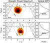 |
Fig. 7 Wavelets for the density signals shown in Fig. 6. Periods are measured in units of t0. |
| In the text | |
|
Fig. 8 Spatial cuts for the axis (top) and wing (bottom). |
| In the text | |
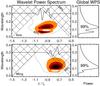 |
Fig. 9 Wavelets for the density signals shown in Fig. 8. |
| In the text | |
|
Fig. 10 Evolution of wing wave train with distance. The signal is plotted at times
|
| In the text | |
|
Fig. 11 Evolution of the trapped wave train. The signals at times
|
| In the text | |
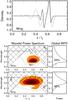 |
Fig. 12 Same as Fig. 11 but for the wing wave train (see also Fig. 10). |
| In the text | |
|
Fig. 13 Wing density signals for Δz of 0.02 (top), 0.1 (middle), and 0.5 (bottom). |
| In the text | |
|
Fig. 14 Density profile for a funnel with density contrast ρF/ρ∞ = 10, p = 8, and no stratification. |
| In the text | |
|
Fig. 15 Density signals and wavelets measured inside (top) and outside (bottom) the funnel density structure for ρF/ρ∞ = 10. |
| In the text | |
|
Fig. 16 Density (top) and Alfvén speed (bottom) profiles for a funnel with density contrast ρF/ρ∞ = 3, p = 8 and stratification with Λeff = 2. The background density has the same vertical stratification, such that the density contrast ratio remains constant with height. |
| In the text | |
|
Fig. 17 Density signals and wavelets measured inside (top) and outside (bottom) the stratified funnel shown in Fig. 16. |
| In the text | |
Current usage metrics show cumulative count of Article Views (full-text article views including HTML views, PDF and ePub downloads, according to the available data) and Abstracts Views on Vision4Press platform.
Data correspond to usage on the plateform after 2015. The current usage metrics is available 48-96 hours after online publication and is updated daily on week days.
Initial download of the metrics may take a while.