| Issue |
A&A
Volume 559, November 2013
|
|
|---|---|---|
| Article Number | A41 | |
| Number of page(s) | 5 | |
| Section | Stellar structure and evolution | |
| DOI | https://doi.org/10.1051/0004-6361/201322353 | |
| Published online | 05 November 2013 | |
Research Note
The first analysis of extragalactic binary-orbit precession ⋆
Astronomical Institute, Charles University in Prague, Faculty of Mathematics and Physics, 180 00 Praha 8, V Holešovičkách 2, Czech Republic
e-mail: This email address is being protected from spambots. You need JavaScript enabled to view it.
Received: 24 July 2013
Accepted: 26 September 2013
Abstract
Aims. The main aim of the present paper is the very first analysis of the binary-orbit precession out of our Galaxy.
Methods. The light curves of an eclipsing binary MACHO 82.8043.171 in the Large Magellanic cloud (LMC) were studied in order to analyse the long-term evolution of its orbit.
Results. It is a detached system that is undergoing rapid orbit precession. The inclination of the orbit towards the observer has been changing, which has caused the eclipse depth to become lower over the past decade, and this is ongoing. The period of this effect was derived as only about 77 years, so it is the second fastest nodal motion known amongst such systems nowadays. This is the first analysis of an extragalactic binary with nodal precession. This effect is probably caused by a distant third body orbiting the pair, which could potentially be detected via spectroscopy.
Conclusions. Some preliminary estimates of this body are presented. However, even such a result can tell us something about the multiplicity fraction in other galaxies.
Key words: binaries: eclipsing / stars: fundamental parameters / stars: individual: MACHO 82.8043.171
Based on data collected with the Danish 1.54 m telescope at the ESO La Silla Observatory.
© ESO, 2013
1. Introduction
After more than a century of intensive study of eclipsing binaries (EBs), they still represent the best method for deriving the masses, radii, and luminosities of stars. Thanks to modern (ground- and space-based) telescopes, we are able to also study these objects in other galaxies and to apply the same methods as used in our solar neighbourhood. Nevertheless, there is still a difference in the precision of EB parameters as derived for Galactic (~2–3%) and extragalactic (~10%) eclipsing binaries (see e.g. Clausen 2004; Ribas 2004).
The extragalactic EBs can serve as an independent tool for deriving Galactic properties and also help us answer such important questions as “Is the chemical composition of our Galaxy the same as the neighbouring ones?” or “What is the binary and multiplicity fraction in other galaxies?”. Studying other galaxies via detailed analysis of individual stars can provide some useful hints for answering these questions.
EBs are quite common, even in some nearby galaxies (Vilardell et al. 2006). However, one special group of EBs is still rather rare – those undergoing an orbit precession. If the orientation of the EB orbit is moving in space, then the depths of eclipse also change, and we can detect this orbit precession. Observing the binary at different time epochs can help us to derive the inclination towards the observer as a function of time. This effect is usually caused by the third component orbiting the close pair (Söderhjelm 1975). However, we still know of only a few such systems, and detailed analysis has only been carried out for those located in our Galaxy at present. This is the first time such an effect has been studied in an extragalactic source.
2. The system MACHO 82.8043.171
The Large Magellanic Cloud (LMC) is a close galaxy, which has been observed quite frequently during the past decades. There have been two major photometric surveys of LMC stars, MACHO (Faccioli et al. 2007) and OGLE (Graczyk et al. 2011), while discovering a huge number of variable stars including the EBs. The MACHO survey lasted from 1993 to 1998 and the OGLE from 2002 to 2008. Quite surprisingly, thanks to these two surveys we know more eclipsing binaries in the LMC than in our Galaxy (Graczyk et al. 2011). However, owing to the low declination of LMC stars, there are still many interesting systems that lack detailed analysis.
The object called MACHO 82.8043.171 (=OGLE-LMC-ECL-17359, V = 16.98 mag) was observed by both photometric surveys, so we can harvest the databases for a complete light curve analysis. The system is a detached eclipsing binary with its short orbital period of about 1.26 day (Graczyk et al. 2011). According to its photometric indices (see below), it is probably a B2V-type system. Our new observations were obtained during a four-month period in the 2012/2013 season, using the 1.54-m Danish telescope located at the La Silla observatory in Chile (hereafter DK154), but operated remotely from the Czech Republic. The standard Cousins filter I was used for our new observations, in agreement with the OGLE survey. Therefore, we can make the first analysis of this interesting system ranging over two decades to detect some long-term changes.
For a complete light curve analysis, we need up-to-date ephemerides of the binary. Using the MACHO and OGLE photometry and deriving the precise times of minima, the following ephemerides were used for the light curve analysis:
 These ephemerides are also suitable for planning future observations. From the observations we determine that the orbit is circular (i.e. no deviation of secondary minima appears).
3. Analysis
The light curve fitting of available photometric data was performed using the program PHOEBE, ver. 0.31a (Prša & Zwitter 2005), which is based on the Wilson-Devinney algorithm (Wilson & Devinney 1971) and its later modifications.
The following procedure was used for the analysis. First, the ephemerides and temperature of the primary component were fixed for the entire computational process. The temperature of the primary component was estimated from its photometric index. Owing to many different sources and a rather wide range of magnitude values for the red and infrared filters, this approach was found to be problematic. For example, the (V − R) photometric index ranges from −0.60 mag (Zacharias et al. 2004) to 0.065 mag (Derekas et al. 2007), which yields a range of spectral types from O to A. On the other hand, Larsen et al. (2000) published the Strömgren uvby photometry, which can be transformed (Harmanec & Božić 2001) into the Johnson UBV system. After these transformations, the unreddened values of the photometric indices (B − V)0 = −0.23 mag resulted, as did (U − B)0 = −0.87 mag, which clearly show the star to be about a B2V spectral type (Golay 1974). Although the star is not single, the two components are rather similar (see below), so we accepted this estimation. The resulting value of E(B − V) = 0.42 mag was quite surprising, because it is a bit larger than commonly used for LMC binaries, but it is still acceptable (Larsen et al. 2000). Another source of Johnson magnitudes is, for example, the one by Zaritsky et al. (2004), who published the UBVI photometry. Regrettably, this photometry is also unusable due to larger errors and unacceptable (U − B)0 values. To conclude, after assuming the B2V spectral type, we fixed the temperature at T1 = 21 000 K (Worthey & Lee 2011) for the computing process.
Owing to rather different quality of the individual light curves, the first OGLE data set (2002.5) was used as the initial one. With this light curve we analysed the system, resulting in a set of parameters for both components, see Table 1. These parameters are the best we were able to derive from the available light curves. The values for temperature, the secondary component, Kopal’s modified potential, luminosities, etc. were used for the subsequent light curve analysis of data obtained at different epochs. However, the lack of other relevant information (e.g. from spectroscopy) meant that some of the parameters have to be fixed for the whole analysis. We assumed a circular orbit (i.e. e = 0) and a mass ratio q = 1. The albedo coefficient remained fixed at value 1.0, gravity darkening coefficients at g = 1.0, and the synchronicity parameters at F = 1. The limb darkening coefficients were interpolated from the van Hamme’s tables (van Hamme 1993). No third light was detected for any of the light curves.
This analysis is based on the assumption that the two components are rather similar to each other. This presumption was derived from the resulting parameters from Table 1 (similar temperatures and luminosities), as well as from the (B − R) photometric index at various orbital phases as derived from the MACHO data. On the other hand, the use of photometry by Larsen et al. (2000) was obtained during many nights of observations, which did not take the current orbital phase of the binary into account, which means that some of the photometric data points could have been obtained during the eclipses. However, no other better photometry is available, and owing to the duration of eclipses (both about 1/10 of the orbital period), only about 20% of the data points are likely to be influenced by the eclipses. However, we still believe that this does not play a significant role because of the similarity of the two eclipsing components. The best way would be to obtain the individual times of observations for the photometry of Larsen et al. (2000), but after communicating with the author, this information is no longer available.
During the fitting process, the mass ratio can also be fitted. As a result, we made this attempt, but it did not result in any significant improvement of the fit. The mass ratio is only poorly constrained here, which agrees with a previous finding that detached eclipsing binaries with only partial eclipses are not suitable for deriving the mass ratio only from the light curves, see e.g. Terrell & Wilson (2005). We can therefore only roughly estimate the uncertainty of the mass ratio to be about 0.1.
A sample of fitted light curve plots at different time epochs is given in Fig. 1. As one can see, the depths of both primary and secondary minima are changing over the two decades. From these fits, the individual inclination angles as derived from the Wilson-Devinney algorithm are given in Table 2 and plotted in Fig. 2. The inclination is seen to change quite fast (more than 2° every year), and the amplitude of photometric variation is rather shallow at present.
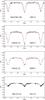 |
Fig. 1 Sample of plots of the light curves at different epochs. Since the range for the y-axis is the same for all plots, the change in amplitude is clearly visible. |
One can also ask how we dealt with the different light curves in different filters for the complete analysis. Our new observations were obtained in the same filter (I) as the OGLE survey. The second OGLE filter (V) was not used because of a limited dataset. On the other hand, both the B and R filters from the MACHO survey were used for the analysis. The light curves in different filters and different epochs were analysed separately, resulting in different inclination angles. These two values of inclination angles (but obtained during the same epoch) were averaged into the value presented in Table 2. We could afford to combine different filters and instruments for the analysis, because the different luminosity levels for different passbands were also computed.
Parameters of the light curve.
Inclination angles as derived from different light curves.
4. Results
The system undergoes a nodal precession of its orbit, which is probably caused by an orbiting third body. This effect of binary orbit precession is nothing new; however, it has been observed and analysed for the first time for an extragalactic source. One can compute the nodal period from the equation given in Söderhjelm (1975): 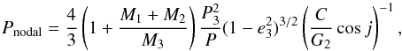 where subscripts 1 and 2 stand for the components of the eclipsing binary, while 3 stands for the third body. The term C is the total angular momentum of the system, while G2 stands for the angular momentum of the wide orbit.
Unfortunately, we are not able to derive the nodal period using this equation owing to unknown individual orbital parameters and masses of the components. We therefore used a simplified approach to fitting the term “cosi”, as given, say, in Drechsel et al. (1994):  where I is the inclination of the invariant plane against the observer’s celestial plane, i is the inclination of the eclipsing binary, and i1 is the inclination between the invariant plane and the orbital plane of the eclipsing binary.
Figure 3 shows the result of our fitting. The resulting nodal period is only about 76.9 ± 10.1 years. However, because of the poor coverage of this period with only two decades of data, this result is still rather preliminary. New and more precise observations (both photometry and spectroscopy) are needed in upcoming years. The resulting period of nodal precession is the second shortest among known systems to date, the fastest motion being that of the well-known system V907 Sco (Lacy et al. 1999) with its nodal period about 68 years. For MACHO 82.8043.171, we do expect that the photometric eclipses will stop as late as about 2017. Until that time only very shallow ellipsoidal variations of the order of 0.03 mag (I filter) remain.
As a by-product we also derived the inclination angles I and i1 from the equation for cosi. These two quantities resulted in I = 41.1° ± 11.8° and i1 = 42.0° ± 13.2°. The values define the orientation of the system in space and towards the observer (see Fig. 2 in Söderhjelm 1975). Both these angles could potentially be used for future dynamical studies, should the third-body orbit be discovered via spectroscopy.
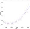 |
Fig. 3 “cosi” term and its final fit (see the text). A confidence level of 95% is shown with the dash-dotted lines. |
5. Discussion
Discovering the nodal precession of MACHO 82.8043.171, one can ask whether the third body causing this effect is detectable with current data or facilities. The easiest method is the light curve analysis and detection of the third light. However, no such additional light was discovered, so that it gives some constraints on this body. Assuming a detection limit of about 1% of the total light, then the undiscovered third component has to be spectral type A2 or later, assuming it lies on the main sequence. We can only speculate about its period and semimajor axis, so that the amplitudes of radial velocity variations are also questionable. The absence of any third light makes it similar to the recently discovered system HS Hya (Zasche & Paschke 2012), where the third body causing the nodal precession of the eclipsing pair also cannot be detected in the light curve solution, but was discovered via spectroscopy.
Moreover, the configuration of the system has to be hierarchical because of its stability (Harrington 1992). Another limiting factor is the fact that any variation in the times of minima is detectable in the O–C diagram of MACHO 82.8043.171 (also analogous to HS Hya). As a result, a detection limit of about 0.002 days also yields some constraints on the third-body orbit, mainly the period, see e.g. Mayer (1990). Using the equation introduced in Söderhjelm (1975), and applying many ad hoc assumptions (e.g. orientation of the orbit in space, fixing the eccentricity to zero), we can roughly estimate, for example, the orbital period of the third component. See Fig. 4 for some results, where the predicted masses (solid curves) and amplitudes of the light-time effect (dash-dotted curves) are plotted with respect to the orbital period P3. The individual colours stand for different inclinations of the orbits: 90° (blue), 70° (black), 50° (red), 30° (cyan), and 10° (green), respectively. Moreover, the dynamical stability criterion also exists, and it gives the lower limit of the third-body period: P/P3 > 5, see e.g. Tokovinin (2008), resulting in a minimum period of about 6.28 days. Considering all these criteria, the shadowed area in Fig. 4 shows the most probable solutions. The expected period P3 should probably be from 6 to 15 days. Moreover, as we can see from Fig. 4, the limit of no detectable period variation of the order of 0.002 day gives a better constraint on the mass of the third body (about 0.4 M⊙) than the absence of the third light, which yields an upper limit of mass of about 2 M⊙. Such a companion is therefore probably an M-dwarf star.
Besides MACHO 82.8043.171, we currently know of only four other systems with derived nodal periods. However, this unique system is the first analysed eclipsing binary with changing inclination outside our own Galaxy. The authors are aware of the most important deficiency of the present analysis, which is the lack of radial velocity measurements, or the detailed spectroscopic study discovering the third component. On the other hand, as we can see, for example, in the system of HS Hya, the third body could have a period of hundreds of days, so to discover it one needs spectroscopic monitoring over several months. Moreover, other EBs within the LMC are much brighter and also have longer periods. There is still no radial velocity study of an LMC eclipsing binary with such a short orbital period. Precise spectroscopic observations for such a faint target would only be possible using 4 m class telescopes or even larger. This first analysis of MACHO 82.8043.171 could serve as a starting point for other astronomers to initiate observing campaigns or to submit observing proposals for this target on large telescopes.
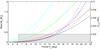 |
Fig. 4 Predicted parameters of the third body resulting from the nodal period. Its period (the x-axis) versus its mass (y-axis, solid curves) is computed from the nodal period, and the corresponding amplitude of the light-time effect was computed (y-axis on the right, dash-dotted curves). The shadowed area represents the possible parameters. Different colours represent different orientations of the orbit in space. See the text for details. |
6. Conclusion
More detailed study of such systems would potentially be very important for several reasons. First, EBs are still the best method for deriving precise masses and radii of stars, and also for calibrating the cosmic distance ladder. Secondly, the chemical compositions of such systems should be studied in order to compare the LMC and our Galaxy. There are some traces of different composition between LMC, SMC, and our Galaxy stars, which were derived using EBs (Ribas 2004). Additionally, the EBs serve as independent distance indicators to the LMC (up to 2%, Pietrzyński et al. 2013). And finally, the changing inclination indicates that there is a hidden component orbiting this EB pair, which could tell us something about the stellar multiplicity of the LMC in general. Observing the suspicious EBs would help us discover these third bodies, which is otherwise rather complicated for such distant objects. (Spectroscopy is time-consuming and magnitude-limited, and interferometry cannot be used for Magellanic clouds.)
Additionally, multiple systems with moving orbital planes are ideal astrophysical laboratories for dynamical studies. The observable quantities can be directly compared with theoretical models. Therefore, each new system is very promising. In our Galaxy we know of 11 such systems nowadays (Zasche & Paschke 2012). Graczyk et al. (2011) noted 17 systems in the LMC, and from the Kepler data there were seven more of these binaries (Rappaport et al. 2013).
Acknowledgments
An anonymous referee is acknowledged for the useful comments and suggestions that significantly improved the paper. Dr. William Hartkopf is also gratefully acknowledged for his help with the language level of the manuscript. We thank the MACHO and OGLE teams for making all of the observations publicly available. We are also grateful to the ESO team in La Silla for their help in maintaining and operating the Danish telescope. This work was supported by the Czech Science Foundation grant no. P209/10/0715, by the grant UNCE 12 of Charles University in Prague, and by the grant LG12001 of the Ministry of Education of the Czech Republic. This research made use of the SIMBAD database, operated at the CDS, Strasbourg, France, and of NASA’s Astrophysics Data System Bibliographic Services.
References
- Clausen, J. V. 2004, New Astron. Rev., 48, 679 [Google Scholar]
- Derekas, A., Kiss, L. L., & Bedding, T. R. 2007, ApJ, 663, 249 [NASA ADS] [CrossRef] [Google Scholar]
- Drechsel, H., Haas, S., Lorenz, R., & Mayer, P. 1994, A&A, 284, 853 [NASA ADS] [Google Scholar]
- Faccioli, L., Alcock, C., Cook, K., et al. 2007, AJ, 134, 1963 [NASA ADS] [CrossRef] [Google Scholar]
- Golay, M. 1974, Introduction to astronomical photometry, Astrophys. Space Sci. Lib., 41 [Google Scholar]
- Graczyk, D., Soszyński, I., Poleski, R., et al. 2011, Acta Astron., 61, 103 [NASA ADS] [Google Scholar]
- Harmanec, P., & Božić, H. 2001, A&A, 369, 1140 [NASA ADS] [CrossRef] [EDP Sciences] [Google Scholar]
- Harrington, R. W. 1992, in IAU Colloq. 135: Complementary Approaches to Double and Multiple Star Research, eds. H. A. McAlister, & W. I. Hartkopf, ASP Conf. Ser., 32, 212 [Google Scholar]
- Lacy, C. H. S., Helt, B. E., & Vaz, L. P. R. 1999, AJ, 117, 541 [NASA ADS] [CrossRef] [Google Scholar]
- Larsen, S. S., Clausen, J. V., & Storm, J. 2000, A&A, 364, 455 [NASA ADS] [Google Scholar]
- Mayer, P. 1990, Bull. Astron. Inst. Czech., 41, 231 [Google Scholar]
- Pietrzyński, G., Graczyk, D., Gieren, W., et al. 2013, Nature, 495, 76 [NASA ADS] [CrossRef] [PubMed] [Google Scholar]
- Prša, A., & Zwitter, T. 2005, ApJ, 628, 426 [NASA ADS] [CrossRef] [Google Scholar]
- Rappaport, S., Deck, K., Levine, A., et al. 2013, ApJ, 768, 33 [NASA ADS] [CrossRef] [Google Scholar]
- Ribas, I. 2004, New Astron. Rev., 48, 731 [Google Scholar]
- Söderhjelm, S. 1975, A&A, 42, 229 [NASA ADS] [Google Scholar]
- Terrell, D., & Wilson, R. E. 2005, Ap&SS, 296, 221 [NASA ADS] [CrossRef] [Google Scholar]
- Tokovinin, A. 2008, MNRAS, 389, 925 [NASA ADS] [CrossRef] [Google Scholar]
- van Hamme, W. 1993, AJ, 106, 2096 [NASA ADS] [CrossRef] [Google Scholar]
- Vilardell, F., Ribas, I., & Jordi, C. 2006, A&A, 459, 321 [NASA ADS] [CrossRef] [EDP Sciences] [Google Scholar]
- Wilson, R. E., & Devinney, E. J. 1971, ApJ, 166, 605 [NASA ADS] [CrossRef] [Google Scholar]
- Worthey, G., & Lee, H.-C. 2011, ApJS, 193, 1 [NASA ADS] [CrossRef] [EDP Sciences] [Google Scholar]
- Zacharias, N., Monet, D. G., Levine, S. E., et al. 2004, BAAS, 36, 1418 [Google Scholar]
- Zaritsky, D., Harris, J., Thompson, I. B., & Grebel, E. K. 2004, AJ, 128, 1606 [NASA ADS] [CrossRef] [Google Scholar]
- Zasche, P., & Paschke, A. 2012, A&A, 542, L23 [NASA ADS] [CrossRef] [EDP Sciences] [Google Scholar]
All Tables
All Figures
|
Fig. 1 Sample of plots of the light curves at different epochs. Since the range for the y-axis is the same for all plots, the change in amplitude is clearly visible. |
| In the text | |
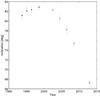 |
Fig. 2 Changing inclination as a function of time. For the explanation of the symbols see Table 2. |
| In the text | |
|
Fig. 3 “cosi” term and its final fit (see the text). A confidence level of 95% is shown with the dash-dotted lines. |
| In the text | |
|
Fig. 4 Predicted parameters of the third body resulting from the nodal period. Its period (the x-axis) versus its mass (y-axis, solid curves) is computed from the nodal period, and the corresponding amplitude of the light-time effect was computed (y-axis on the right, dash-dotted curves). The shadowed area represents the possible parameters. Different colours represent different orientations of the orbit in space. See the text for details. |
| In the text | |
Current usage metrics show cumulative count of Article Views (full-text article views including HTML views, PDF and ePub downloads, according to the available data) and Abstracts Views on Vision4Press platform.
Data correspond to usage on the plateform after 2015. The current usage metrics is available 48-96 hours after online publication and is updated daily on week days.
Initial download of the metrics may take a while.