| Issue |
A&A
Volume 559, November 2013
|
|
|---|---|---|
| Article Number | A100 | |
| Number of page(s) | 9 | |
| Section | Atomic, molecular, and nuclear data | |
| DOI | https://doi.org/10.1051/0004-6361/201321893 | |
| Published online | 21 November 2013 | |
Energy levels and transition rates for the boron isoelectronic sequence: Si X, Ti XVIII – Cu XXV⋆,⋆⋆
1 Group for Materials Science and Applied Mathematics, Malmö
University, Sweden
e-mail:
per.jonsson@mah.se
2
Vilnius University, Institute of Theoretical Physics and
Astronomy, A. Goštauto
12, 01108
Vilnius,
Lithuania
3
Chimie Quantique et Photophysique, CP160/09, Université Libre de
Bruxelles, Av. F.D. Roosevelt
50, 1050
Brussels,
Belgium
4
Department of Electrical Engineering and Computer
Science, Box
1679B, Vanderbilt
University, TN 37235, USA
Received:
14
May
2013
Accepted:
14
July
2013
Relativistic configuration interaction (RCI) calculations are performed for 291 states belonging to the configurations 1s22s22p, 1s22s2p2, 1s22p3, 1s22s23l, 1s22s2p3l, 1s22p23l, 1s22s24l′, 1s22s2p4l′, and 1s22p24l′ (l = 0,1,2 and l′ = 0,1,2,3) in boron-like ions Si X and Ti XVIII to Cu XXV. Electron correlation effects are represented in the wave functions by large configuration state function (CSF) expansions. States are transformed from jj-coupling to LS-coupling, and the LS-percentage compositions are used for labeling the levels. Radiative electric dipole transition rates are given for all ions, leading to massive data sets. Calculated energy levels are compared with other theoretical predictions and crosschecked against the Chianti database, NIST recommended values, and other observations. The accuracy of the calculations are high enough to facilitate the identification of observed spectral lines.
Key words: atomic data / atomic processes
Research supported in part by the Swedish Research council and the Swedish Institute. Part of this work was supported by the Communauté française of Belgium, the Belgian National Fund for Scientific Research (FRFC/IISN Convention) and by the IUAP-Belgian State Science Policy (BriX network P7/12).
Tables of energy levels and transition rates (Tables 3–19) are only available at the CDS via anonymous ftp to cdsarc.u-strasbg.fr (130.79.128.5) or via http://cdsarc.u-strasbg.fr/viz-bin/qcat?J/A+A/559/A100
© ESO, 2013
1. Introduction
The X-ray spectra from L-shell ions are particularly important for astrophysics, as they are in the wavelength range covered by telescopes on board the space observatories Chandra and XMM-Newton (Landi & Gu 2006). The analysis of high-resolution X-ray spectra requires knowledge of energy levels and a large number of accurate transition rates, either from theory or experiment, to identify spectral lines, produce synthetic spectra, and carry out plasma diagnostics. Similarly, spectra from these ions find applications in the diagnostics and modeling of fusion plasmas. The work on fusion plasma is especially important in relation to the International Thermonuclear Experimental Reactor (ITER).
During the past few years a number of calculations have been carried out to provide more complete sets of energies and transition data for L-shell ions. Merkelis et al. (1995) used the stationary second-order many-body perturbation theory (MBPT) to compute energies for n = 2 levels, and transition rates for boron-like ions for Z = 8 to 26. The relativistic effects in those calculations were accounted for in the Breit-Pauli approximation. Safronova et al. (1996, 1998, 1999) used relativistic many-body perturbation theory (RMBPT) to compute energies for n = 2, 3 levels and transition rates between n = 2 states for boron-like ions with nuclear charges ranging from Z = 5 to 100. Gu (2005a) used relativistic configuration interaction and many-body perturbation theory to compute energies of n = 2 levels for ions with Z ≤ 60. The work was later extended to levels in boron-like iron and nickel involving higher n (Gu 2005b, 2007). The calculations by Safronova et al. and Gu are highly accurate and in many cases, give transition wavelengths to within a few mÅ, comparable to what can be obtained in experimental work. Results with high accuracy were obtained by Rynkun et al. (2012) using relativistic configuration interaction (RCI). Energies for n = 2 levels and E1, M1, and E2 transition rates were reported for ions with Z = 7 to 30. Vilkas et al. (2005) used relativistic multireference many-body perturbation theory (MRMP) to calculate energies in Si X. The energies were accurate enough to unambiguously identify EUV and soft-X-ray spectral lines in old beam-foil spectra. The combined theoretical and experimental work resulted in an extensive data set that is suitable for the validation of different computational methods.
Much work has been focused on iron. Landi & Gu (2006) used the flexible atomic structure code (FAC) to calculate energy levels, transition rates, and electron-ion excitation collision strengths for high-energy configurations in the iron ions Fe XVII to Fe XXIII. Massive calculations have recently also been performed by Jonauskas et al. (2006) and Nahar (2010). These calculations include hundreds of fine-structure levels, but the accuracy of the computed energies is not as high as for the calculations by Safronova et al. (1996, 1998), Gu (2005b, 2007), and Rynkun et al. (2012).
Although theoretical data are available, it is still very difficult to analyze spectra, unambiguously identify transitions, and deduce energy levels with the proper labels. Looking at the NIST Atomic Spectra Database (2013), there remain large gaps that need to be filled and misidentifications are present. This paper reports on RCI calculations for 291 states belonging to the configurations 1s22s22p, 1s22s2p2, 1s22p3, 1s22s23l, 1s22s2p3l, 1s22p23l, 1s22s24l′, 1s22s2p4l′, and 1s22p24l′ (l = 0, 1,2 and l′ = 0, 1,2,3) in boron-like ions Si X, and Ti XVIII to Cu XXV. Energy levels and electric dipole transition rates between the states are given. Results are crosschecked and validated against other theoretical predictions and experimental data. The work is part of a long-term theoretical effort to attain spectroscopic accuracy, i.e. calculated transition energies that are accurate enough to directly confirm or revise experimental identifications. It complements and extends previous work on boron-, carbon-, nitrogen-, oxygen-, and neon-like systems, where energies have been provided with relative inaccuracies of fractions of a per mille (Rynkun et al. 2012; Jönsson et al. 2011, 2013a).
2. Relativistic multiconfiguration calculations
The calculations were performed using the fully relativistic multiconfiguration Dirac-Hartree-Fock (MCDHF) method in jj-coupling (Grant 2007). For practical purposes, a transformation from jj- to LS-coupling (Gaigalas et al. 2003) was done at the end, and in all tables, the quantum states are labeled by the leading LS-percentage composition.
2.1. Multiconfiguration Dirac-Hartree-Fock
Starting from the Dirac-Coulomb Hamiltonian,
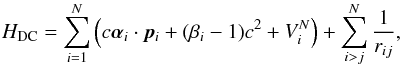 (1)where
VN is the monopole part of the
electron-nucleus Coulomb interaction, α and
β the 4 × 4 Dirac matrices, and c the speed of light
in atomic units, the atomic state functions were obtained as linear combinations of
symmetry adapted configuration state functions (CSFs):
(1)where
VN is the monopole part of the
electron-nucleus Coulomb interaction, α and
β the 4 × 4 Dirac matrices, and c the speed of light
in atomic units, the atomic state functions were obtained as linear combinations of
symmetry adapted configuration state functions (CSFs): 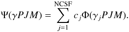 (2)Here, J
and M are the angular quantum numbers and P is the
parity. The label γj denotes other
appropriate information of the configuration state function j, such as
orbital occupancy and coupling scheme. The CSFs were built from products of one-electron
Dirac orbitals. Based on a weighted energy average of several states known as the extended
optimal level (EOL) scheme (Dyall et al. 1989), both
the radial parts of the Dirac orbitals and the expansion coefficients were optimized to
self-consistency in the relativistic self-consistent field (RSCF) procedure.
(2)Here, J
and M are the angular quantum numbers and P is the
parity. The label γj denotes other
appropriate information of the configuration state function j, such as
orbital occupancy and coupling scheme. The CSFs were built from products of one-electron
Dirac orbitals. Based on a weighted energy average of several states known as the extended
optimal level (EOL) scheme (Dyall et al. 1989), both
the radial parts of the Dirac orbitals and the expansion coefficients were optimized to
self-consistency in the relativistic self-consistent field (RSCF) procedure.
The transverse interaction in the low-frequency limit, or the Breit interaction (McKenzie et al. 1980), ![\begin{equation} \label{eq:Breit} H_{\mbox{{\footnotesize Breit}}} = - \sum_{i<j}^N \frac{1}{2 r_{ij}} \Biggl[ \bm{\alpha}_{i} \cdot \bm{\alpha}_{j} + \frac{ (\bm{\alpha}_{i} \cdot {\bm{ r_{ij} }}) (\bm{\alpha}_{j} \cdot {\bm{ r_{ij} }}) } {r_{ij}^2} \Biggr], \end{equation}](/articles/aa/full_html/2013/11/aa21893-13/aa21893-13-eq34.png) (3)and leading QED (vacuum
polarization and self-energy) were included in subsequent configuration interaction (RCI)
calculations. All calculations were performed with the GRASP2K code (Jönsson et al. 2007, 2013b). To
calculate the spin-angular part of the matrix elements, the second quantization method in
coupled tensorial form and quasispin technique (Gaigalas et
al. 1997) was adopted.
(3)and leading QED (vacuum
polarization and self-energy) were included in subsequent configuration interaction (RCI)
calculations. All calculations were performed with the GRASP2K code (Jönsson et al. 2007, 2013b). To
calculate the spin-angular part of the matrix elements, the second quantization method in
coupled tensorial form and quasispin technique (Gaigalas et
al. 1997) was adopted.
2.2. Transition parameters
The evaluation of spontaneous transition rates, A, between two states,
γ′P′J′M′
and γPJM, built on different and independently optimized orbital sets is
non-trivial. The transition rates, or probabilities, can be expressed in terms of the
transition moment, which is defined as
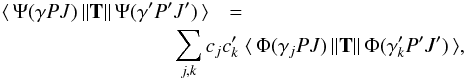 (4)where
T is the transition operator (Cowan
1981). The calculation of the transition moment breaks down to the task of
summing up reduced matrix elements between different CSFs. The reduced matrix elements can
be evaluated using standard techniques assuming that both left and right hand CSFs are
formed from the same orthonormal set of spin-orbitals. This constraint is
severe, since a high-quality and compact wave function requires orbitals optimized for
specific electronic states from which orbital non-orthogonalities arise in the calculation
of transition amplitudes (Fritzsche et al. 1994). To
get around the problems, the wave functions of the two states,
γ′P′J′M′
and γPJM, were separately optimized, and their representations were
transformed in such a way that the orbital sets became biorthonormal (Olsen et al. 1995). Standard methods were then used to
evaluate the matrix elements between the transformed CSFs.
(4)where
T is the transition operator (Cowan
1981). The calculation of the transition moment breaks down to the task of
summing up reduced matrix elements between different CSFs. The reduced matrix elements can
be evaluated using standard techniques assuming that both left and right hand CSFs are
formed from the same orthonormal set of spin-orbitals. This constraint is
severe, since a high-quality and compact wave function requires orbitals optimized for
specific electronic states from which orbital non-orthogonalities arise in the calculation
of transition amplitudes (Fritzsche et al. 1994). To
get around the problems, the wave functions of the two states,
γ′P′J′M′
and γPJM, were separately optimized, and their representations were
transformed in such a way that the orbital sets became biorthonormal (Olsen et al. 1995). Standard methods were then used to
evaluate the matrix elements between the transformed CSFs.
For electric dipole (E1) transitions, there are two forms of the transition operator, the length, and velocity form (Grant 1974). The length form is usually the preferred one. The agreement between transition rates computed in the two forms can be used as an indicator of the accuracy of the underlying wave functions (Froese Fischer 2009). In this work, we introduce the ratio, R, between the transition rates, A, in length and velocity forms as the indicator.
2.3. Validation for Si X
Si X holds a prominent position among boron-like ions because many energy levels are known with a high accuracy from the combined theoretical and experimental work by Vilkas et al. (2005). The ion is thus an excellent testing ground. To validate current computational methods and strategies, calculations were performed for the lowest states belonging to the configurations 1s22s22p, 1s22s2p2, 1s22p3, 1s22s23l, 1s22s2p3l, and 1s22p23l (l = 0,1,2) in Si X. We describe the calculations for the odd states. The calculations for the even parity states were done in a similar manner.
As a starting point, an RSCF calculation was performed in the EOL scheme for the weighted average of the odd parity reference states. To include electron correlation, this calculation was followed by two calculations where the CSF expansions were obtained by allowing single and double (SD) excitations from all shells of the odd parity reference configurations to active orbital sets with principal quantum numbers up to n = 4 and 5, respectively. Additional RSCF calculations were performed for CSF expansions obtained by allowing SD excitations from the outer shells of the odd reference configurations to active orbital sets that were systematically enlarged from n = 6 up to n = 9 and with orbital angular momenta up to l = 6. The RSCF calculations generated a well balanced active orbital set. In a final step, an RCI calculation was performed. The expansion was obtained by allowing SD excitations from all shells of the reference configurations to the largest active orbital set. The resulting expansion that accounted for core-core, core-valence, and valence-valence electron correlation effects consisted of 474 000 CSFs distributed over the J = 1/2,3/2,...,9/2 angular symmetries. The same computational strategy applied to the even parity states yielded a final RCI expansion that consisted of 503 000 CSFs. Tests indicated that the calculated properties were well converged with respect to the active orbital sets.
2.4. Calculations for Ti XVIII to Cu XXV
For the ions Ti XVIII to Cu XXV, that is the focus of this paper, we considered the levels belonging to the configurations 1s22s22p, 1s22s2p2, 1s22p3, 1s22s23l, 1s22s2p3l, 1s22p23l, 1s22s24l′, 1s22s2p4l′, and 1s22p24l′ (l = 0, 1,2 and l′ = 0,1, 2,3). The calculations for these ions were done in a similar way as for Si X, generating active orbital sets with orbitals up to n = 9 and l = 6. The final RCI calculations were based on expansions obtained by allowing SD excitations from all shells of the reference configurations to the largest active orbital sets. Due to a larger number of reference states for Ti XVIII to Cu XXV, as compared with Si X, the expansions were now larger. For the odd parity states, there were 982 000 CSFs distributed over the J = 1/2,3/2,...,11/2 angular symmetries. For the even parity states, there were 971 000 CSFs. For Ti XVIII to Cu XXV, the orbital set spans more states compared with Si X. However, tests indicated that the calculated properties were well converged with respect to the active orbital sets also in this case.
2.5. Labeling of states
The wave functions in the present work were obtained as expansions over jj-coupled CSFs, and it is convenient to give the states the same labels as the dominating CSFs. The states were, however, not well described in jj-coupling, and in the expansions, many CSFs had nearly the same weight. To adhere to the labeling in the NIST database and in other sources, the states should instead be given in LS-coupling. As discussed by Safronova et al. (1998), LS-coupling is neither a good labeling system nor is it straightforward to assign labels. Safronova et al. (1998) used a number of rules to perform the task, but these were sometimes not consistent with the experimental labels, thus, causing confusion. In this work, we used a module in the latest release of the GRASP2K code (Jönsson et al. 2013b) to transform from jj- to LS-coupling to obtain the leading LS-percentage composition. This gave a label system compatible with the one used by experimentalists, which often relied on calculations using the HFR suite of codes Cowan (1981) for their analysis. It also corresponded to the labels obtained from non-relativistic calculations with relativistic corrections in the Breit-Pauli approximation (Jonauskas et al. 2006; Nahar 2010). It should be noted that there were also states with the same leading LS-percentage composition in LS-coupling, and for these states, a more complete composition should be used as the label.
3. Results and discussion
3.1. Energies for Si X
The calculations for Si X serve as validation. In Table 1, we compare energies in Si X from the final RCI calculation with observed and
calculated energies by Vilkas et al. (2005) and
from the Chianti database (Landi et al. 2012). The
calculations by Vilkas et al. are based on relativistic multireference many-body
perturbation theory (MRMP). The experimental energies in the Chianti database are all
reassessed from the original wavelength measurements. There are, however, only small
differences compared with the experimental energies given by Vilkas et al. The theoretical
energies given in the Chianti database are from R-matrix calculations by Liang et al. (2009). In Table 1, there are also energies from RMBPT calculations by Safronova et al. (1996, 1998). Labels from the latter calculations in some cases did not match the
labels from the RCI calculations. From the J quantum number and the
computed energies, it was however possible to correctly match all the levels. Except for
the R-matrix calculation that was optimized for electron-ion collisional data, which
requires a comparatively small target, there is an excellent agreement between the
different sets of calculations and observations. The mean relative energy differences
between calculations and observations are 0.018% for RCI, 0.029% for MRMP, and 0.068% for
RMBPT. Looking at Table 1 more closely, it is seen that two many-body perturbation
theory-based calculations (MRMP and MBPT) yield values that are too low, but the third
(RMBPT) yields values that are too high. To quantify this, we computed the mean level
deviation (MLD) between the observed and calculated energy levels. The MLD is given by
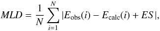 (5)where
the energy shift (ES) is chosen to minimize the sum. The MLD and ES are 236
cm-1 and 12 cm-1 for RCI, 258 cm-1 and − 47
cm-1 for MRMP, and 770 cm-1 and 804 cm-1 for RMBPT.
Although not very large, there is a positive bias of the predicted energy levels from the
RMBPT calculations.
(5)where
the energy shift (ES) is chosen to minimize the sum. The MLD and ES are 236
cm-1 and 12 cm-1 for RCI, 258 cm-1 and − 47
cm-1 for MRMP, and 770 cm-1 and 804 cm-1 for RMBPT.
Although not very large, there is a positive bias of the predicted energy levels from the
RMBPT calculations.
Energies in cm-1 for levels in Si X.
Energies in cm-1 for levels in Fe XXII.
3.2. Energies for Fe XXII
In Table 2, we give calculated energies for the levels belonging to the configurations 1s22s22p, 1s22s2p2, 1s22p3, 1s22s23l, 1s22s2p3l, and 1s22p23l (l = 0,1,2) in Fe XXII. The full data set comprising of levels with n = 4 is given in Table 7. In Table 2, calculated and observed energies from the Chianti database (Landi et al. 2012) are also given. Calculated energies held by the Chianti database are from Landi & Gu (2006). The observed levels are from different sources and all the references are given in the database. In addition, energies from RMBPT calculations by Safronova et al. (1996, 1998) and (Gu 2005b, 2007) are given. Due to inconsistencies in the labels, the RMBPT results by Safronova et al. (1996, 1998) in several cases were matched using J quantum numbers and computed energies. There is an excellent agreement between the energies from the RCI calculations and the RMBPT calculations. Similar to Si X, the energies from the RMBPT calculations are higher than the energies from the RCI calculations. The agreement with the calculated energies from the Chianti database (Landi et al. 2012) is very good but not on the same level as for the RMBPT calculations. In most cases, there is a satisfactory agreement with the observed energies. The lack of experimental data, however, makes it difficult to distinguish between different theories, and we need to fall back on the results from Si X to draw any conclusions about the accuracy of the calculated energies. Undoubtedly, the combined energy levels from the RCI and RMBPT calculations provide a very good starting point for further identifications of observed lines.
3.3. Energies for Ti XVIII to Cu XXV
In Tables 3–10, energies from the RCI calculations are given for the levels belonging to the configurations 1s22s22p, 1s22s2p2, 1s22p3, 1s22s23l, 1s22s2p3l, 1s22p23l, 1s22s24l′, 1s22s2p4l′, and 1s22p24l′ (l = 0,1,2 and l′ = 0,1,2,3) in boron-like ions from Ti XVIII to Cu XXV. Energy levels are given in cm-1 relative to the ground state 1s22s22p 2P1/2. In addition, the LS-percentage compositions obtained by transforming from jj- to LS-coupling are displayed. It should be carefully noted that some excited levels have the same leading LS-percentage, and in this case, an extended composition should be used as a label. One example is levels 62 and 63 in Fe XXII that are given as 0.41 2p2(3P)3s 4P + 0.39 2s2p(1P)3p 2S + 0.07 2p2(1S)3s 2S and 0.46 2p2(3P)3s 4P + 0.42 2s2p(1P)3p 2S + 0.07 2s2p(1P)3p 2P, respectively. Further, it should be noted that levels of the form 1s22s25l start to show up far up in the spectra, where the energy separation is small. These levels were not specifically targeted in the RCI calculations, and it is not known how well they are described. The calculated energies are compared with recommended data from the NIST Atomic Spectra Database (2013) and from the Chianti database for Fe XXII (Landi et al. 2012). The original references are as follows: Ti XVIII, Mn XXI (Sugar & Corliss 1985); V XIX, Cr XX, Co XXIII, Ni XXIV (Sugar & Corliss 1985; Shirai et al. 2000); Cu XXV (Sugar & Musgrove 1990). There is a detailed agreement between calculations and observed energies for the n = 2 levels. Observed energies for the more excited levels are lacking to a large extent. For the few available levels and for some ions such as Cr XX, there is good agreement between the calculated and observed energies. However, there are a number of individual levels where theory and experiment can not be reconciled.
Validations in Si X and Fe XXII show that the energies from the RCI calculations are highly accurate. The energies thus serve as benchmarks for other calculations. They are also valuable in further experimental work, both for Fe XXII and for the other ions, as a means to unambiguously identify spectral lines.
3.4. Transition rates
In Table 11, transition rates, A, between the n = 2 states in Fe XXII are displayed. In addition, there are some transitions including states with n = 3. For the RCI calculations, the ratio R of the transition rates in length and velocity gauges are also shown. The ratio R is used to assess the accuracy of the transition rates. For highly accurate wave functions and strong transitions, R should be close to 1. Values far from 1 indicate that there may be internal cancellations, and weak transitions with values of R far from 1 are generally associated with larger uncertainties. For a deeper discussion about error estimates, see Froese Fischer (2009). The transition rates are compared with values from RMBPT calculations by Safronova et al. (1999), from MBPT calculations by Merkelis et al. (1995), and with values from calculations by Landi & Gu (2006) that are part of the Chianti database. There is a much better consistency between the current rates and the rates by Merkelis et al. (1995) and Landi & Gu (2006) than there is with Safronova et al. (1999); the relative differences being less than 5% for the first two, whereas it is 14% for the RMBPT. Rates from RCI calculations have previously been carefully validated against experiments and other accurate calculations for ions in the boron isoelectronic sequence (Rynkun et al. 2012). In the studied ions, there was an agreement between different calculations at the 1% level. We thus argue that the current rates represent an improvement in accuracy compared with available data in the Chianti databases and to the RMBPT calculations by Safronova et al. (1999).
In Tables 12–19, transition energies, wavelengths, transition rates A, weighted oscillator strengths gf, and the ratio R of the transition probabilities in length and velocity gauges are displayed for transitions in Ti XVIII to Cu XXV. The transition rates between the n = 2 states agree very well with the previous RCI calculations by Rynkun et al. (2012). Many of the transitions with R far from 1 involve configurations that differ by two or more electrons such as 2s23p–2s2p2 (transition 17–8 in Table 16) or 2s2p3d–2p23s (transition 71–65 in Table 16). These transitions are forbidden in the single configuration approximation and are opened due to configuration interaction. The rates of these transitions are extremely challenging to compute, and for some of them, the values from various calculations differ substantially. These type of transitions have recently been analyzed by Bogdanovich et al. (2007).
4. Conclusions
We have used large scale RCI calculations with expansion sizes of nearly a million CSFs to obtain transition energies for levels belonging to the configurations 1s22s22p, 1s22s2p2, 1s22p3, 1s22s23l, 1s22s2p3l, 1s22p23l, 1s22s24l′, 1s22s2p4l′, and 1s22p24l′ (l = 0,1,2 and l′ = 0,1,2,3) in boron-like ions from Ti XVIII to Cu XXV. The problem of labeling has been discussed, and we used a transformation from jj- to LS-coupling to obtain the leading LS-percentage compositions. The latter are used as labels for the levels. Computational methods and strategies have been validated for Si X, where accurate energies are available (Vilkas et al. 2005). For Si X, energies from the RCI calculations are in excellent agreement with observations with a mean relative energy difference of only 0.018%. For Fe XXII, the calculated energies are checked against values from the Chianti database (Landi et al. 2012), RMBPT calculations by Safronova et al. (1996, 1998) and Gu (2005b, 2007), and from MBPT calculations by Merkelis et al. (1995). There is a detailed agreement between the present energies and the energies from the RMBPT calculations. In most cases, there is also a good agreement with observations. However, there are obvious cases where theory and experiment do not match at all. The agreement is also very good between the present energies and the experimental energies for the n = 2 levels of ions other than Fe XXII. For these ions, experimental energies for higher levels are largely missing. For the energies that are available, most notably in Cr XX, there is a good consistency with the energies from the RCI calculations in many cases. However, there are several cases where there are obvious experimental misidentifications. The present energies are the most accurate energies available for these ions. They should be of value for future experimental work.
A comparison of the transition rates between the n = 2 states in Fe XXII shows that the values are less consistent than could originally be expected. The current transition rates differ from the RMBPT values by 14%, but the agreement is better for the stronger transitions. The agreement with the calculations by Merkelis et al. (1995) and Landi & Gu (2006) is considerably better with a relative difference of around 5%. Rates from RCI calculations have previously been carefully validated against experiments and other accurate calculations for ions in the boron isoelectronic sequence. Rates in the studied ions agreed between different calculations at the 1% level (Rynkun et al. 2012). We thus argue that the current rates represent an improvement in accuracy compared with available data in the Chianti database and from the RMBPT and MBPT calculations by Safronova et al. (1999) and Merkelis et al. (1995).
References
- Bogdanovich, P., Karpuškienė, R., & Rancova, O. 2007, Phys. Scr., 75, 669 [NASA ADS] [CrossRef] [Google Scholar]
- Cowan, R. 1981, The theory of atomic structure and spectra (Berkeley: University of California Press) [Google Scholar]
- Dyall, K. G., Grant, I. P., Johnson, C. T., Parpia, F. A., & Plummer, E. P. 1989, Comput. Phys. Commun., 55, 425 [NASA ADS] [CrossRef] [Google Scholar]
- Fritzsche, S., & Grant, I. P. 1994, Phys. Lett. A, 186, 152 [NASA ADS] [CrossRef] [Google Scholar]
- Froese Fischer, C. 2009, Phys. Scr., 134, 014019 [Google Scholar]
- Gaigalas, G., Rudzikas, Z., & Froese Fischer, C. 1997, J. Phys. B At. Mol. Opt. Phys., 30, 3747 [Google Scholar]
- Gaigalas, G., Žalandauskas, T., & Rudzikas, Z. 2003, At. Data Nucl. Data Tables, 84, 99 [NASA ADS] [CrossRef] [Google Scholar]
- Grant, I. P. 1974, J. Phys. B, 7, 1458 [Google Scholar]
- Grant, I. P. 2007, Relativistic Quantum Theory of Atoms and Molecules (New York: Springer) [Google Scholar]
- Gu, M. F. 2005a, At. Data Nucl. Data Tables, 89, 267 [NASA ADS] [CrossRef] [Google Scholar]
- Gu, M. F. 2005b, ApJSS, 156, 105 [NASA ADS] [CrossRef] [Google Scholar]
- Gu, M. F. 2007, ApJSS, 169, 154 [NASA ADS] [CrossRef] [Google Scholar]
- Jonauskas, V., Bogdanovich, P., Keenan, F. P., et al. 2006, A&A, 455, 1157 [NASA ADS] [CrossRef] [EDP Sciences] [Google Scholar]
- Jönsson, P., He, X., Froese Fischer, C., & Grant, I. P. 2007, Comput. Phys. Commun., 177, 597 [NASA ADS] [CrossRef] [MathSciNet] [Google Scholar]
- Jönsson, P., Rynkun, P., & Gaigalas, G. 2011, At. Data Nucl. Data Tables, 97, 648 [Google Scholar]
- Jönsson, P., Bergtsson, P., Ekman, J., et al. 2013a, At. Data Nucl. Data Tables, in press, http://dx.doi.org/10.1016/j.adt.2013.06.001 [Google Scholar]
- Jönsson, P., Gaigalas, G., Bieroń, J., Froese Fischer, C., & Grant, I. P. 2013b, Comput. Phys. Commun., 184, 2197 [NASA ADS] [CrossRef] [Google Scholar]
- Kramida, A., Ralchenko, Yu., Reader, J., & NIST ASD Team 2012, NIST Atomic Spectra Database (ver. 5.0), National Institute of Standards and Technology, http://physics.nist.gov/asd [Google Scholar]
- Landi, E., & Gu, M. F. 2006, ApJ, 640, 1171 [NASA ADS] [CrossRef] [Google Scholar]
- Landi, E., Del Zanna, G., Young, P. R., et al. 2012, ApJS, 744, 99 [NASA ADS] [CrossRef] [Google Scholar]
- Liang, G. Y., Whiteford, A. D., & Badnell, N. R. 2009, A&A, 499, 943 [NASA ADS] [CrossRef] [EDP Sciences] [Google Scholar]
- McKenzie, B. J., Grant, I. P., & Norrington, P. H. 1980, Comput. Phys. Commun., 21, 233 [NASA ADS] [CrossRef] [Google Scholar]
- Merkelis, G., Vilkas, M. J., Gaigalas, G., & Kisielius, R. 1995, Phys. Scr., 51, 233 [NASA ADS] [CrossRef] [Google Scholar]
- Nahar, S. N. 2010, At. Data Nucl. Data Tables, 96, 26 [NASA ADS] [CrossRef] [Google Scholar]
- Olsen, J., Godefroid, M., Jönsson, P., Malmqvist, P. Å., & Froese Fischer, C. 1995, Phys. Rev. E, 52, 4499 [NASA ADS] [CrossRef] [Google Scholar]
- Rynkun, P., Jönsson, P., Gaigalas, G., & Froese Fischer, C. 2012, At. Data Nucl. Data Tables, 98, 481 [Google Scholar]
- Safronova, M. S., Johnson, W. R., & Safronova, U. I. 1996, Phys. Rev. A, 54, 2850 [NASA ADS] [CrossRef] [PubMed] [Google Scholar]
- Safronova, U. I., Johnson, W. R., & Safronova, M. S. 1998, At. Data Nucl. Data Tables, 69, 183 [NASA ADS] [CrossRef] [Google Scholar]
- Safronova, U. I., Johnson, W. R., & Livingston, A. E. 1999, Phys. Rev. A, 60, 996 [NASA ADS] [CrossRef] [Google Scholar]
- Shirai, T., Sugar, J., Musgrove, A., & Wisese, W. L. 2000, J. Phys. Chem. Ref. Data, Monograph, 8, 1 [NASA ADS] [Google Scholar]
- Sugar, J., & Corliss, C. 1985, J. Phys. Chem. Ref. Data, 14, Suppl. 2, 1 [Google Scholar]
- Sugar, J., & Musgrove, A. 1990, J. Phys. Chem. Ref. Data, 19, 527 [NASA ADS] [CrossRef] [Google Scholar]
- Vilkas, M., Ishikawa, Y., & Träbert, E. 2005, Phys. Scr., 72, 181 [NASA ADS] [CrossRef] [Google Scholar]
All Tables
Current usage metrics show cumulative count of Article Views (full-text article views including HTML views, PDF and ePub downloads, according to the available data) and Abstracts Views on Vision4Press platform.
Data correspond to usage on the plateform after 2015. The current usage metrics is available 48-96 hours after online publication and is updated daily on week days.
Initial download of the metrics may take a while.