| Issue |
A&A
Volume 559, November 2013
|
|
|---|---|---|
| Article Number | A21 | |
| Number of page(s) | 8 | |
| Section | Stellar structure and evolution | |
| DOI | https://doi.org/10.1051/0004-6361/201321849 | |
| Published online | 30 October 2013 | |
The fundamental parameters of the roAp star 10 Aquilae⋆
1
Institut d’Astrophysique et de Planétologie de Grenoble, CNRS-UJF UMR
5571,
414 rue de la Piscine, 38400
St Martin d’Hères
France
2
Centro de Astrofísica e Faculdade de Ciências, Universidade do
Porto, 4150-762
Porto,
Portugal
3
Laboratoire Lagrange, UMR 7293 UNS-CNRS-OCA, Boulevard de
l’Observatoire, BP
4229, 06304
Nice Cedex 4,
France
4
Georgia State University, PO Box 3969, Atlanta
GA
30302-3969,
USA
5
CHARA Array, Mount Wilson Observatory,
91023
Mount Wilson
CA,
USA
Received: 6 May 2013
Accepted: 9 August 2013
Abstract
Context. Owing to the strong magnetic field and related abnormal surface layers existing in rapidly oscillating Ap (roAp) stars, systematic errors are likely to be present when determining their effective temperatures, which potentially compromises asteroseismic studies of this class of pulsators.
Aims. Using the unique angular resolution provided by long-baseline visible interferometry, our goal is to determine accurate angular diameters of a number of roAp targets, so as to derive unbiased effective temperatures (Teff) and provide a Teff calibration for these stars.
Methods. We obtained long-baseline interferometric observations of 10 Aql with the visible spectrograph VEGA at the combined focus of the CHARA array. We derived the limb-darkened diameter of this roAp star from our visibility measurements. Based on photometric and spectroscopic data available in the literature, we estimated the star’s bolometric flux and used it, in combination with its parallax and angular diameter, to determine the star’s luminosity and effective temperature.
Results. We determined a limb-darkened angular diameter of 0.275 ± 0.009 mas and deduced a linear radius of R = 2.32 ± 0.09 R⊙. For the bolometric flux we considered two datasets, leading to an effective temperature of Teff = 7800 ± 170 K and a luminosity of L/L⊙ = 18 ± 1 or Teff = 8000 ± 210 K and L/L⊙ = 19 ± 2. Finally we used these fundamental parameters together with the large frequency separation determined by asteroseismic observations to constrain the mass and the age of 10 Aql, using the CESAM stellar evolution code. Assuming a solar chemical composition and ignoring all kinds of diffusion and settling of elements, we obtained a mass M/M⊙ ~ 1.92 and an age of ~780 Gy or a mass M/M⊙ ~ 1.95 and an age of ~740 Gy, depending on the derived value of the bolometric flux.
Conclusions. For the first time, thanks to the unique capabilities of VEGA, we managed to determine an accurate angular diameter for a star smaller than 0.3 mas and to derive its fundamental parameters. In particular, by only combining our interferometric data and the bolometric flux, we derived an effective temperature that can be compared to those derived from atmosphere models. Such fundamental parameters can help for testing the mechanism responsible for the excitation of the oscillations observed in the magnetic pulsating stars.
Key words: methods: observational / techniques: high angular resolution / techniques: interferometric / stars: individual: 10 Aql / stars: fundamental parameters
Based on observations made with the VEGA/CHARA spectro-interferometer.
© ESO, 2013
1. Introduction
Rapidly oscillating Ap (roAp) stars are a subgroup of Ap stars that are chemically peculiar main-sequence magnetic stars of spectral type B8 to F0. The roAp stars exhibit strong large-scale organized magnetic fields (between a hundred of G up to 24.5 kG for HD 154708 – Hubrig et al. (2005)), abundance anomalies ofSr, Cr and rare earths, small rotation speeds (≤100 km s-1 and often ≤30–40 km s-1), and pulsations with a range of amplitudes from about 10 millimagnitudes (Kurtz et al. 2006) to 10 micromagnitudes (Balona et al. 2011) and periods ranging from 6 min for HD 134214 (Saio et al. 2012) up to 24 min for HD 177765 (Alentiev et al. 2012). These pulsations are interpreted as high-order, low-degree acoustic modes.
The mechanism inducing the slow rotation of these stars is likely due to magnetic braking. Stȩpień (2000) concludes that this magnetic braking must occur during the pre-main sequence phase so as to reproduce the angular momentum observations of the Ap stars. This theory is corroborated by the recent study of the rotation of magnetic Herbig AeBe stars by Alecian et al. (2013). In addition, several spectro-polarimetric observations of Herbig AeBe provide evidence of magnetic fields whose strength and topology are similar to those of Ap stars (Wade et al. 2007; Alecian et al. 2008). This seems to indicate that magnetic Herbig AeBe stars are the progenitors of Ap stars.
In (ro)Ap stars, the strong magnetic field is supposed to play a key role in the abundance distribution by stabilizing the external layers and partially or fully suppressing the convection. Vertical and horizontal microscopic diffusion of the chemical elements (Michaud 1970) is thus believed to occur, leading to spotted surfaces that have been reconstructed by Doppler or Zeeman-Doppler imaging for several (ro)Ap stars (Lüftinger et al. 2003, 2010; Kochukhov et al. 2004; Kochukhov & Wade 2010). Such abnormal surface layers might generate systematic errors when determining stellar luminosities and effective temperatures by spectrometric or photometric techniques (Matthews et al. 1999).
For a long time it was considered that such a strong magnetic field prevented oscillations from existing. But in 1978, 12-min oscillations were first detected in the Ap Przybylski’s star (Kurtz 1978) which became the first roAp star. Up to now, more than 40 roAp have been discovered. Their oscillations are different from those observed in the other types of pulsating stars that lie in the instability strip of the Hertzsprung-Russell (HR) diagram (like δ-Scuti, γ-Dor, and Cepheids stars). While the periods of the roAp oscillations are analogous to those of the solar ones (supposed to come from the Lighthill process), their amplitudes cover a much wider range. The mechanism responsible for the excitation of the oscillations observed in roAp stars is still a matter of debate. Currently the most promising theory is that envelope convection is suppressed by the strong magnetic fields present in these stars and excitation then occurs as a result of the opacity mechanism acting on the convectively stable hydrogen ionization zone (Balmforth et al. 2001). This hypothesis has been tested with reasonable success through nonadiabatic calculations (Cunha 2002). Moreover, microscopic diffusion is also supposed to have a significant impact on the excitation process (Théado et al. 2005).
Deriving accurate fundamental parameters of a large sample of roAp stars is of strong interest for comparing both adiabatic and nonadiabatic model predictions with observations. Creevey et al. (2007) and Cunha et al. (2007) have shown that an accurate linear radius provided by interferometry combined with asteroseismic data allows an accurate stellar mass to be derived and stellar interiors to be tested: typically an accuracy better than 3% on the radius allows an accuracy better than 4% to be reached on the mass. With the recent operation of visible interferometers working on very long-baseline arrays like VEGA on the CHARA array (Mourard et al. 2009), the angular resolution is now of the order of 0.2 millisecond of arc (mas), which allows resolving several roAp stars despite their very small angular size (i.e. ≤1 mas). Up to now, the angular diameters of three roAp stars have been determined by optical interferometry: a limb-darkened angular diameter of 1.105 ± 0.037 mas for α Cir with SUSI (Bruntt et al. 2008), limb-darkened angular diameters of 0.669 ± 0.017 mas and 0.415 ± 0.017 mas for the two components of β CrB with FLUOR (Bruntt et al. 2010), and a limb-darkened angular diameter of 0.564 ± 0.017 mas for γ Equ with VEGA (Perraut et al. 2011). These angular diameters have been used to derive the stars’ effective temperatures and differences between these interferometric effective temperatures and the photometric effective temperatures have been highlighted.
Thanks to the unique capabilities of VEGA in terms of high angular resolution, we can extend this sample to smaller roAp stars. We present here the results we obtained on 10 Aql (HD 176232; F0p), which is one of the brightest roAp stars of the northern hemisphere (mV ~ 5.9). Its parallax is well known, πP = 12.76 ± 0.29 mas (van Leeuwen 2007). Its rotation period is unknown but it might be of several hundreds of years, given its rotation speed vsini less than 2.0 ± 0.5 km s-1 (Kochukhov et al. 2002). Ryabchikova et al. (2000) and, more recently, Nesvacil et al. (2013) have studied the abundances of this target. Ryabchikova et al. (2000) detect strong overabundances in doubly ionized elements of rare earths (like neodymium or praseodymium), while Nesvacil et al. (2013) derive a self-consistent, chemically stratified atmosphere model for 10 Aql. Elements Mg and Co were found to be the least stratified, while Ca and Sr exhibited the largest abundance stratifications. Kochukhov et al. (2002) have measured a mean magnetic field modulus of ⟨ B ⟩ = 1.5 ± 0.1 kG in 10 Aql from Zeeman splitting.
This star was discovered as a roAp by Heller & Kramer (1988) with a pulsation period of about 11.9 min and an amplitude well below one millimagnitude. Huber et al. (2008) continuously followed this target with the MOST satellite during one month for identifying the pulsation frequencies and studying the effect of the magnetic field. Even if the frequency spectrum was found to not be rich enough to allow the authors to converge towards a unique model, they could derive a large frequency separation of Δν = 50.95 μHz and show that the best fit corresponds to a 1.95 M⊙ model having solar metallicity, suppressed envelope convection, and homogenous helium abundance.
In this paper, we report our interferometric observations of 10 Aql with the VEGA instrument (Sect. 2), which allow a limb-darkened angular diameter to be derived. To fix the star’s position in the HR diagram, we compute the star’s bolometric flux (Sect. 3) and derive its fundamental parameters (Sect. 4). We then use a stellar evolution code to determine the mass and the age of the target (Sect. 5). Finally, we discuss how our results compare with those published in the literature (Sect. 6).
2. Interferometric observations and data processing
2.1. CHARA/VEGA observations
Log of the observations.
The CHARA array (ten Brummelaar et al. 2010) hosts six one-meter telescopes arranged in a Y shape and oriented to the east (E1 and E2), south (S1 and S2) and west (W1 and W2). The baselines B span between 30 m (S1S2) and 330 m (S1W1) allowing a maximal angular resolution of λ/(2B) ~ 0.2 mas to be reached in the visible range. The VEGA spectrograph is one of the visible focal instruments of the array. It can combine 2, 3, or 4 telescopes, and it allows recording spectrally dispersed fringes from 0.45 μm to 0.85 μm at a spectral resolution of 6000 (medium resolution) or 30 000 (high resolution) as described in Mourard et al. (2009). VEGA is equipped with two photon-counting detectors looking at two different spectral bands. In the medium spectral resolution, these two bands have spectral bandwiths of 30 nm for the shortest observed wavelengths and 40 nm for the longest ones. The two bands are separated by about 170 nm. The medium spectral resolution is used for diameter determination via squared visibility measurements. This mode reaches a limiting correlated magnitude of mV ~ 6.5 in medium seeing conditions. The high spectral resolution is used for kinematics studies via differential observable measurements. The limiting correlated magnitude is then mV ~ 4.5.
VEGA can be operated in parallel with the CLIMB beam combiner working in the K band and acting as a coherence sensor (Sturmann et al. 2010). In this near-infrared range, the turbulence is less penalizing and the fringe contrast is higher since the angular resolution is smaller. CLIMB can thus ensure the necessary fringe stability required for the long observing sequences in the visible. We measured a typical residual jitter on the optical path difference on the order of 7 μm, which is in good agreement with our need in medium spectral resolution (20 μm).
We have observed 10 Aql with different telescope triplets chosen to partially resolve the small expected angular diameter of the target (about 0.3 mas, so close to the angular resolution limit of VEGA). The spectral bands were centered on 550 nm and 720 nm. For the shorter wavelengths, only the excellent seeing conditions allow the visibility to be retrieved. We followed a sequence calibrator-target-calibrator, with 40 or 60 blocks of 1000 short exposures (of 25 ms) per star. Swapping from one star to another every 20 or 30 min ensures that the instrumental transfer function is stable enough. We used the SearchCal software (Bonneau et al. 2006) proposed by the JMMC1 to find two relevant calibrators for our target: HD 170878 and HD 160765. Their uniform-disk angular diameters are determined by surface-brightness versus color-index relationships. An accuracy of 7% on the angular diameter is obtained by using the (V, V − K) polynomial relation. This leads to a uniform-disk angular diameter in the R band of 0.242 ± 0.017 mas for HD 170878 and of 0.151 ± 0.011 mas for HD 160765. The observation log is given in Table 1, and the corresponding spatial frequency (u, v) coverage is displayed to the left in Fig. 1.
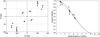 |
Fig. 1 Left. Spatial frequency coverage of the VEGA observations. Right. Squared visibility versus spatial frequency for 10 Aql obtained with the VEGA observations (diamonds). The solid line and the open circles represent the uniform-disk best model provided by LITPRO. |
2.2. VEGA data processing
The interferometric data were reduced using the standard VEGA reduction pipeline described in Mourard et al. (2009). This software allows computing the squared visibility in wide spectral bands based on the spectral density analysis. For each night, we first checked that the instrumental transfer function is stable over the night by computing this function transfer for all the calibrators of all the programs of the night as explained in Mourard et al. (2012). Bad sequences due to poor seeing conditions or instrumental instabilities noted in the journal of the night were rejected.
For each data sequence (calibrator-target-calibrator), we computed the raw squared visibility for each block of 1000 individual frames and for different spectral bands of 20 nm (whose central wavelengths λ0 are given in Table 1). Such large bandwidths lead to an effective spectral resolution of 36 (at the optical wavelength of VEGA), which means that our visibility measurements are mainly sensitive to the continuum (or photosphere) of the star. The individual spectral lines of 10 Aql are indeed unresolved at such a spectral resolution (Fig. 2).
Using the known angular diameter of the calibrators, we calibrated the target squared visibilities V2 and estimated a weighted-mean calibrated squared visibility and the corresponding errors that were twofold: σstat was derived from the statistical dispersion over the block’s measurements, and σsyst accounted for the uncertainty on the calibrator diameter. For each target sequence, we then studied the influence of selecting the individual block’s squared visibility on a signal-to-noise ratio (S/N) criterion. We determined the threshold on S/N where the estimated calibrated visibility started to be biased. Under good seeing conditions, putting a high S/N threshold does not change the mean value of the squared visibilities and only decreases the statistical dispersion σstat, as for the data of May 2012. However, for average or bad seeing conditions, putting a high S/N threshold tends to increase the squared visibilities and bias the measurements. Such a trend clearly appeared for the data recorded in September 2011 with a r0 of 6–7 cm. For such seeing conditions we could only retrieve unbiased squared visibilities for the shortest baseline (i.e., for the most contrasted fringes).
From this study of our measurement bias, we decided to consider furthermore the values of the calibrated squared visibilities obtained for a S/N threshold of four and discarded the biased visibilities. We kept 15 visibility points whose values are given in Table 1. For baselines up to about 200 m the error on the squared visibilities is dominated by the statistical dispersion (σstat is 3 or 4 times larger than σsyst), while for the longest baseline (i.e., more than 300 m), it can be dominated by the accuracy on the calibrators’ diameter. This is the case for the excellent data of May 2012 where σsyst is twice greater than σstat for the E1W1 baseline.
 |
Fig. 2 Spectrum of 10 Aql at the medium spectral resolution of VEGA (~6000). Each visibility measurement is computed over a 20-nm range. |
 |
Fig. 3 Spectral energy distribution obtained for 10 Aql using the dataset described in case 1 (left panel) and the dataset described in case 2 (right panel). In both plots, the IUE spectrum is shown in black at the lower wavelengths, the STIS spectrum is shown in blue, the interpolations are shown in gray and the 2MASS data are shown by orange circles. In addition, in the right panel, the ELODIE spectrum is shown in yellow, the Kurucz model at the higher wavelengths is shown in black and the Breger data are shown by purple stars. (See online edition for a color version.) |
2.3. Deriving a uniform-disk angular diameter
We plotted all the calibrated squared visibilities as a function of the spatial frequency (Bp/λ) and performed a model fitting using LITpro (Tallon-Bosc et al. 2008) proposed by the JMMC2. This fitting engine is based on a modified Levenberg-Marquardt algorithm combined with the trust region method. The software provides a user-expandable set of geometrical elementary models of the object, combinable as building blocks. The fit of all the visibility measurements versus spatial frequency leads to a uniform-disk angular diameter θUD of 0.264 ± 0.0085 mas for 10 Aql (Fig. 1-right). We check the effect of the wavelength by independently fitting the visibility measurements corresponding to 730−735 nm (8 visibility points) and to 695–715 nm (7 visibility points). The angular diameter we obtain at 730–735 nm is slightly larger than the one at 695–715 nm, but the difference (less than 1-σ) is not significant compared to the error bars. Moreover, both values are also consistent with the result from the global fit. On the other hand, owing to the (u, v) coverage (Fig. 1-left), we only probe one baseline direction (around −105° ± 15°), and we cannot determine any angular diameter variation with respect to the baseline orientation. As a consequence, we consider all measurements as a whole and fix θUD of 0.264 ± 0.0085 mas in the following.
2.4. Deriving a limb-darkened angular diameter
The tables of Diaz-Cordoves et al. (1995) provide the linear limb-darkening coefficients u(λ) in the R, I, J, H, and K bands used to determine the limb-darkened angular diameter in the corresponding band. We derived the limb-darkened angular diameter θLD of 10 Aql in the R band through the formula  (1)where u(R) denotes the limb-darkening coefficient in the R band. It is obtained by the adjustment of the radial intensity distribution on the stellar disk using a stellar atmosphere model characterized by the effective temperature (Teff), the gravity (log g), and the metallicity ([Fe/H]). For a given log g, we computed the coefficients u(R) and the corresponding limb-darkened diameters when the effective temperature spans from 7250 K to 8250 K. We tested three different log g: 3.5, 4, and 4.5. Over these huge temperature and gravity ranges, the limb-darkened diameter only varies by 1.2 × 10⁻³ mas for log g equal to 4 and 4.5 and of 1.7 × 10⁻³ mas for log g = 3.5. We also tested different metallicities from –5 to +1: over this range the limb-darkened diameter only varies of 10-3 mas. These variations are 5–7 times smaller than our error bar on the uniform-disk diameter. We fixed u(R) = 0.505 (for Teff = 7750 K, log g = 4, and a solar metallicity) and obtained a limb-darkened angular diameter of θLD = 0.275 ± 0.009 mas (i.e., about 3% of relative accuracy). To our knowledge, this corresponds to the smallest angular diameter ever measured.
3. Computation of the bolometric flux
To determine the fundamental parameters of 10 Aql, in particular its effective temperature and luminosity, we need to compute the star’s bolometric flux, in addition to the stellar angular diameter derived in Sect. 2.2. This, in turn, requires knowledge about the star’s spectral energy distribution.
3.1. Data
The apparent flux distribution for 10 Aql was obtained by combining photometric and spectroscopic data available in the literature. Since a significant amount of data is available, part of which overlapping in wavelength, we considered two different data combinations for deriving the bolometric fluxes, which provided an indication of uncertainties not accounted for in the individual data measurements.
For the first flux distribution, hereafter case 1, we considered the following data.
-
For wavelengths in the range1150 Å < λ < 3349 Å, we used two rebinned spectra from the Sky Survey Telescope obtained at the IUE “Newly Extracted Spectra” (INES) data archive3. Based on the quality flag listed in the IUE spectra ( Garhart et al. 1997), we removed all bad pixels from the data, and we also removed the measurements with negative flux.
-
For wavelengths in the range 3349 Å < λ < 10 198 Å, we used a low-dispersion STIS spectra extracted from the Next Generation Spectral Library (NGSL), 2nd version4.
-
At longer wavelengths, we collected the photometric data from the 2MASS All Sky Catalog of point sources 5 ( Cutri et al. 2003 ). Filter responses and zeropoints were taken from Cohen et al. (2003) .
For the second flux distribution, hereafter case 2, we considered the same data as above for the shorter wavelengths in the range 1150 Å < λ < 3900 Å, as well as for the longer wavelengths covered by the 2MASS photometry. For wavelengths in between, the data above were replaced by the following data:
-
For wavelengths in the range3900 Å < λ < 6370 Å, we used a flux-calibrated ELODIE spectra extracted from the ELODIE.3.1 library6 (Prugniel & Soubiran 2001; Prugniel et al. 2007).
-
For wavelengths between 6370 Å and 8800 Å, we collected spectrophotometric data from Breger (1976) .
In both cases we performed linear interpolations (on logarithmic scale) between the photometric data points, as well as at both extremes of the spectral distribution, namely between 912 Å and 1150 Å, considering zero flux at 912 Å, and between 21 590 Å and 1.6 × 10⁶ Å, considering zero flux at 1.6 × 10⁶ Å.
3.2. Determination of fbol
The bolometric flux, fbol, was then computed from the integral of the spectral energy distribution found for each case. The spectral energy distributions are shown in Fig. 3, and the corresponding bolometric fluxes are presented in Table 2, as are the uncertainties in the two values of the bolometric flux. These uncertainties were estimated by considering the uncertainties quoted in the data sources (when observed calibrated spectra are used), and a conservative uncertainty of 15% (when interpolations or extrapolations are made). In particular, the uncertainties quoted in the references cited above led us to take 10% uncertainty on the flux component computed from the combined IUE spectra, 3% uncertainty on the flux component computed from the STIS spectrum, and 2.5% uncertainty on the flux component computed from the ELODIE spectrum.
The contributions from the extremes of the spectral distribution (corresponding to extrapolations) were found to account for less than 1% of the total flux. Moreover, we have checked that the use of interpolation between photometric data is adequate by comparing, for case 2, the flux obtained through the approach described above with the flux obtained when using, for wavelengths larger than 6370 Å, a Kurucz model computed with ATLAS9 (Castelli & Kurucz 2003) chosen to fit the star’s spectrum in the visible and the stars’ photometry in the infrared (see previous works, e.g., for details Huber et al. 2012). The relative difference in the fluxes obtained through these two procedures for case 2 was found to be smaller than 3%, so, well within the computed uncertainties.
Fundamental parameters computed for 10 Aql from two datasets and assuming a solar chemical composition (see text for details).
4. Determination of the fundamental parameters
4.1. Linear radius
From a simple Monte Carlo simulation, we derived the radius of 10 Aql and its error thanks to the formula 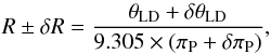 (2)where R stands for the stellar radius (in solar radius, R⊙), θLD for the limb-darkened angular diameter (in mas), and πP for the parallax (in seconds of arc). We obtained R = 2.32 ± 0.09 R⊙. Our accuracy determination of 3.3% on the angular diameter coupled with the well-known parallax (at a 2.3%-precision level) allows us to reach an accuracy of 3.9% on the radius determination.
4.2. Effective temperature and luminosity
We used the measured angular diameter and bolometric flux to estimate the effective temperature from the definition, 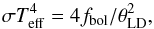 (3)where σ stands for the Stefan-Boltzmann constant (5.67 × 10⁻⁵ erg cm-2 s-1 K-4).
The star’s luminosity was computed by combining the parallax and bolometric flux, through the relation,  (4)where C is the conversion from parsecs to cm (3.086 × 10¹⁸), assuming the bolometric flux is given in cgs units. The values derived for the effective temperature and luminosity for each case considered are shown in Table 2. The corresponding error bars are derived from analytical expressions.
The derivation of a precise value for the effective temperature of 10 Aql was found to be somewhat compromised by the difficulty in establishing a precise value for the bolometric flux of the star. A similar situation was already found for the case of the roAp star γ Equ (Perraut et al. 2011) and is mainly due to the limited quality of flux-calibrated spectra available in the literature. As an example, in the present case of 10 Aql, the STIS spectra used in case 1 was acquired with the star offset from slit center by more that 0.9 pixels. According to the notes published in the NGSL library site4, in this case the slit throughput correction applied to the spectra is unreliable. On the other hand, in case 2, the ELODIE spectrum used in replacement of the STIS spectrum, for wavelengths longer than 3900 Å, does not have the best quality flag for the flux calibration (having a flag of 2 in a scale where the best is 3 and the worst is 0). Given the difficulty in establishing which of the derived bolometric fluxes is the most reliable, we compute evolutionary tracks for both cases.
 |
Fig. 4 The evolutionary tracks corresponding to the case 1 (left) and case 2 (right) are represented with the observational error box (the 1σ-error box (log Teff, log L) in red and the diagonal dotted lines for R). The mass (in solar units) is indicated at the beginning of the evolutionary tracks. In each case, the best model is shown as full line, whereas the two extreme models are shown as dashed lines. For the best model, we show in brackets for several time steps (open circles) the evolution of the mean large separation (μHz), the radius (R⊙), and the age (Gy). The full circles represent the time at which the large separation equals the observed one, i.e. 50.9 μHz. (See online edition for a color version.) |
5. Stellar evolution modeling
We used the stellar evolution code CESAM (Morel 1997; Morel & Lebreton 2008) to derive the mass and the age of the star. The code solves the 1D equations of the quasi-hydrodrostatic stellar evolution coupled with the detailed OPAL equation of state (Rogers et al. 1996) and opacities (Rogers & Iglesias 1992). The nuclear pp- and CNO-reaction rates are determined through the NACRE (Angulo 1999) tables. The convection is treated using the Canuto & Mazzitelli (1991) formalism. The stellar evolution models are coupled with MARCS (Gustafsson et al. 2008) model atmospheres as external boundary conditions. Neither chemical element diffusion nor rotation are taken into account in the calculations. Owing to the strong stratification of the chemical elements into the atmospheres of these magnetic stars, the chemical composition is still a matter of debate. However, spectro-photometry observation can be reproduced well with solar metallicity (Ryabchikova et al. 2000). Moreover, Huber et al. (2008) have explored several cases of chemical mixture for 10 Aql and found that the solar one reproduces spectro-photometric data well. Therefore, following these authors, we decided to use a solar chemical mixture: Z/X = 0.024 and Y = 0.276. Each stellar model is then defined by its mass, age, and convection parameters.
To derive accurate masses and ages, we took advantage of 10 Aql being a multiperiodic pulsator (Huber et al. 2008), which therefore allows the determination of the large frequency separation Δν between eigenmodes of consecutive radial orders. This quantity scales as the square root of the mean density of the star  and therefore decreases as the star evolves. Its value has been accurately derived for 10 Aql by Huber et al. (2008) using the data from the MOST space mission. They find Δν = 50.95 ± 0.03 μHz. The magnetic field creates a shift in the frequencies and therefore affects the large separation. Bigot & Weiss (2002) calculated large separations for a field strength of 800 G, close to the upper limit of 1 kG suggested by Ryabchikova et al. (2000). Even if such a value of the magnetic field strength leads to a shift in frequency in a few μHz, the relative effect between two consecutive modes is weak ~0.1−0.3 μHz and therefore does not influence the derived mass and age, which are mainly constrained by the observational error box in effective temperature, luminosity, and radius.
We considered a null overshoot parameter and various masses between 1.8 and 2.2 M⊙. We kept the stellar models whose evolutionary tracks pass through the observational error box [Teff,log L] and whose mean large separation was equal to the observed one. For our fixed chemical composition, we found two different values of the mass depending on the case considered: 1.92 ± 0.03 M⊙(case 1) and 1.95 ± 0.05 M⊙(case 2). These values of masses and ages (given in Table 2) and especially their uncertainties must be taken with care considering the standard stellar (nonmagnetic) evolution models used in this paper and the fixed choice of chemical mixture (Z/X,Y).
6. Discussion and conclusion
By benefiting from the long CHARA baselines and the visible range of the VEGA instrument, we managed to determine an accurate angular diameter for a target smaller than 0.3 mas. Even though 10 Aql is at the angular resolution limit of VEGA, we reach an accuracy of about 3% on the angular diameter since the recorded fringe contrast is high enough (V2 ≥ 0.4) with hectometric baselines. Using the well-known parallax we derived a linear radius of R = 2.32 ± 0.09 R⊙. From the spectroscopic data, we computed 10 Aql’s bolometric flux and derived its effective temperature (7800–8000 K), luminosity (18 or 19 L⊙), and mass (1.92–1.95 M⊙). All these values can be compared to the previous determinations found in the literature.
As regards to the luminosity, the values we derived in this work are in full agreement with those determined by Nesvacil et al. (2013). These luminosities are slightly lower than those derived from Kochukhov & Bagnulo (2006), who found 21.4 L⊙. This may be due to the bolometric correction adopted by the authors, which was assumed to be the same as for normal stars. Nevertheless, the difference between these values of luminosity is within the error bars.
The masses we derived agree with those found by Huber et al. (2008) (1.95 M⊙), either by calculations from the observed large frequency separation or by model fits based on the pulsation frequencies. But they are larger than those derived in Nesvacil et al. (2013), based on their values of log g and R, which span from 1.4 to 1.7 M⊙ according to the spectrophotometric data set they considered.
From their spectroscopic data and the Warsaw-New Jersey stellar evolution and pulsation code (Pamyatnykh et al. 1998), and assuming a luminosity of 21.4 L⊙ (Matthews et al. 1999), Ryabchikova et al. (2000) derived a mass of 2.0 ± 0.2 M⊙ and two values for the stellar radius, depending on the chosen effective temperature: R = 2.50 ± 0.2 R⊙ for Teff = 7550 K, and R = 2.38 ± 0.2 R⊙ for Teff = 7760 K, respectively. This led them to log g = 3.95 ± 0.25 and log g = 3.99 ± 0.25, respectively. They finally adopted Teff = 7550 K and log g = 3.99 ± 0.25 (and thus R = 2.50 ± 0.2 R⊙) since these values were found to reproduce all the observations best. Their values for the radius agree with our linear radius of R = 2.32 ± 0.09 R⊙. Using the same effective temperature (Teff = 7550 K), Nesvacil et al. (2013) constructed a self-consistent model atmosphere for 10 Aql based on a surface gravity of log g = 3.8. When fitting their model to spectrophotometric observations, the authors derived a linear radius spanning from 2.59 R⊙ to 2.72 R⊙, depending on the assumed atmospheric chemistry (in particular, whether the model is He-solar or He-weak). When their model atmosphere was instead fitted to STIS data (i.e., identical to those considered in (case 2) of Sect. 3), the authors found, for an effective temperature of Teff = 7550 K, a slightly smaller radius of 2.46 ± 0.06 R⊙, which is still more than the value derived here. Concerning the effective temperatures, while our determinations (7800–8000 K) agree with the determination of Kochukhov & Bagnulo (2006) based on photometric data (7925 K), we show a clear discrepancy between our effective temperatures and those adopted either by Ryabchikova et al. (2000) or Nesvacil et al. (2013). Based on spectro-photometry analysis (and especially on the fit of the Paschen continuum), they considered an effective temperature of about 7550 K in their modeling, which is significantly smaller than our determination.
Such discrepancies between the spectroscopic and the interferometric radii and temperatures have been already pointed out in the past for previous studies of roAp stars like β CrB, α Cir, and γ Equ. In all these cases the radii (respectively, effective temperature) derived from optical interferometry were larger (respectively, lower) than those derived from spectroscopic methods (Shulyak et al. 2013), which goes the opposite direction from the case of 10 Aql shown in this work. In addition, we carefully checked our systematic errors, such as the calibrator diameter effect, as well as the dependence of our determination on log g, metallicity, and wavelength. As regards wavelength dependency, the angular diameter seemed to be larger (at less than 1-σ) at shorter wavelengths (around 700 nm), but this trend needs to be confirmed by more accurate data, since we do not have enough visibility measurements to derive accurate angular diameters as a function of wavelength. Our poor (u,v) coverage meant we could not studied the effect of the baseline orientation. It would be very difficult to detect an asymmetry of the angular diameter even with a richer (u,v) coverage because of the very small angular size of the target. As a consequence, it is likely that the discrepancy between our radius and the one derived from atmosphere models is related to model ingredients, so clearly a deeper modeling of 10 Aql is required. Determining accurate and precise fundamental parameters of these complex stars by a method that is as independent as possible of an atmosphere model is thus an efficient way to improve the latter.
Finally, we want to point out that the discrepancy is less than 2σ on the radius, while there are significant differences found in spectroscopic and photometric determinations of the global parameters of roAp stars, and large differences in effective temperature determined by spectroscopy using models with and without stratification of the elements. For instance, for α Cir, Kupka et al. (1996) determine 7900 K, while a recent determination by Kochukhov et al. (2009) gives 7500 K. Indeed, models of atmospheres of Ap stars are extremely complex, and the consequent determination of effective temperature (hence radius, assuming one knows the luminosity) by spectroscopic data is subject to major difficulties. A good way to test the different effective temperatures is to use them as input for excitation models since the excitation region is very sensitive to the temperature. Such a study is in progress (Cunha et al. 2013). A byproduct of these works would be a calibration of the effective temperature scale for these peculiar pulsating stars.
This work emphasizes the potential of combining interferometric (radius and derived effective temperature) and asteroseismic (large frequency separation) data to improve determination of the mass and the age of stars, as already pointed out by Creevey et al. (2007). Our results also clearly demonstrate the feasibility of our roAp program on CHARA/VEGA and the strong interest of increasing the number of targets in our sample. For this program on small targets (usually smaller than 0.5 mas) with the current operational interferometric facilities, only visible long-baseline interferometry can bring accurate angular diameters, and all instrumental improvements towards better sensitivity and better accuracy are of utmost importance.
Available at www.jmmc.fr/searchcal
Acknowledgments
The authors are grateful to Denis Shulyak for fruitful discussions concerning computing the bolometric flux. VEGA is supported by the French programs for stellar physics and high angular resolution PNPS and ASHRA, by the Nice Observatory, and the Lagrange Department. The CHARA Array is operated with support from the National Science Foundation through grant AST-0908253, the W. M. Keck Foundation, the NASA Exoplanet Science Institute, and from Georgia State University. This work has been supported by a grant from LabEx OSUG@2020 (Investissements d’avenir – ANR10LABX56) and made use of funds from the ERC through the project FP7-SPACE-2012-312844. M.C. acknowledges financial support from the FCT through the grant SFRH/BPD/84810/2012. This research made use of the SearchCal and LITPRO services of the Jean-Marie Mariotti Center, and of CDS Astronomical Databases SIMBAD and VIZIER.
References
- Alecian, E., Catala, C., Wade, G. A., et al. 2008, MNRAS, 385, 391 [NASA ADS] [CrossRef] [Google Scholar]
- Alecian, E., Wade, G. A., Catala, C., et al. 2013, MNRAS, 429, 1027 [NASA ADS] [CrossRef] [Google Scholar]
- Alentiev, D., Kochukhov, O., Ryabchikova, T., et al. 2012, MNRAS, 421, L82 [NASA ADS] [Google Scholar]
- Angulo, C. 1999, in AIP Conf. Ser., 495, 365 [Google Scholar]
- Balmforth, N. J., Cunha, M. S., Dolez, N., Gough, D. O., & Vauclair, S. 2001, MNRAS, 323, 362 [NASA ADS] [CrossRef] [Google Scholar]
- Balona, L. A., Cunha, M. S., Kurtz, D. W., et al. 2011, MNRAS, 410, 517 [NASA ADS] [CrossRef] [Google Scholar]
- Bigot, L., & Weiss, W. W. 2002, Commun. Asteroseismol., 141, 26 [NASA ADS] [Google Scholar]
- Bonneau, D., Clausse, J.-M., Delfosse, X., et al. 2006, A&A, 456, 789 [NASA ADS] [CrossRef] [EDP Sciences] [Google Scholar]
- Breger, M. 1976, ApJS, 32, 7 [NASA ADS] [CrossRef] [Google Scholar]
- Bruntt, H., North, J. R., Cunha, M., et al. 2008, MNRAS, 386, 2039 [NASA ADS] [CrossRef] [Google Scholar]
- Bruntt, H., Kervella, P., Mérand, A., et al. 2010, A&A, 512, A55 [NASA ADS] [CrossRef] [EDP Sciences] [Google Scholar]
- Canuto, V. M., & Mazzitelli, I. 1991, ApJ, 370, 295 [NASA ADS] [CrossRef] [Google Scholar]
- Castelli, F., & Kurucz, R. L. 2003, Modelling of Stellar Atmospheres, eds. N. Piskunov et al., IAU Symp., 210, poster A20 [Google Scholar]
- Cohen, M., Wheaton, W. A., & Megeath, S. T. 2003, AJ, 126, 1090 [NASA ADS] [CrossRef] [Google Scholar]
- Creevey, O. L., Monteiro, M. J. P. F. G., Metcalfe, T. S., et al. 2007, ApJ, 659, 616 [NASA ADS] [CrossRef] [Google Scholar]
- Cunha, M. S. 2002, MNRAS, 333, 47 [NASA ADS] [CrossRef] [Google Scholar]
- Cunha, M. S., Aerts, C., Christensen-Dalsgaard, J., et al. 2007, A&ARv, 14, 217 [NASA ADS] [CrossRef] [Google Scholar]
- Cunha, M., Alentiev, D., Brandao, I., & Perraut, K. 2013, MNRAS, in press [Google Scholar]
- Cutri, R. M., Skrutskie, M. F., van Dyk, S., et al. 2003, VizieR Online Data Catalog, II/246 [Google Scholar]
- Diaz-Cordoves, J., Claret, A., & Gimenez, A. 1995, A&AS, 110, 329 [NASA ADS] [Google Scholar]
- Garhart, M. P., Smith, M. A., Turnrose, B. E., Levay, K. L., & Thompson, R. W. 1997, IUE NASA Newsletter, 57, 1 [NASA ADS] [Google Scholar]
- Gustafsson, B., Edvardsson, B., Eriksson, K., et al. 2008, A&A, 486, 951 [NASA ADS] [CrossRef] [EDP Sciences] [Google Scholar]
- Heller, C. H., & Kramer, K. S. 1988, PASP, 100, 583 [NASA ADS] [CrossRef] [Google Scholar]
- Huber, D., Saio, H., Gruberbauer, M., et al. 2008, A&A, 483, 239 [NASA ADS] [CrossRef] [EDP Sciences] [Google Scholar]
- Huber, D., Ireland, M. J., Bedding, T. R., et al. 2012, ApJ, 760, 32 [NASA ADS] [CrossRef] [Google Scholar]
- Hubrig, S., Nesvacil, N., Schöller, M., et al. 2005, A&A, 440, L37 [NASA ADS] [CrossRef] [EDP Sciences] [Google Scholar]
- Kochukhov, O., & Bagnulo, S. 2006, A&A, 450, 763 [NASA ADS] [CrossRef] [EDP Sciences] [Google Scholar]
- Kochukhov, O., & Wade, G. A. 2010, A&A, 513, A13 [NASA ADS] [CrossRef] [EDP Sciences] [Google Scholar]
- Kochukhov, O., Landstreet, J. D., Ryabchikova, T., Weiss, W. W., & Kupka, F. 2002, MNRAS, 337, L1 [NASA ADS] [CrossRef] [Google Scholar]
- Kochukhov, O., Drake, N. A., Piskunov, N., & de la Reza, R. 2004, A&A, 424, 935 [NASA ADS] [CrossRef] [EDP Sciences] [Google Scholar]
- Kochukhov, O., Shulyak, D., & Ryabchikova, T. 2009, A&A, 499, 851 [NASA ADS] [CrossRef] [EDP Sciences] [Google Scholar]
- Kupka, F., Ryabchikova, T. A., Weiss, W. W., et al. 1996, A&A, 308, 886 [NASA ADS] [Google Scholar]
- Kurtz, D. W. 1978, Information Bulletin on Variable Stars, 1436, 1 [Google Scholar]
- Kurtz, D. W., Elkin, V. G., Cunha, M. S., et al. 2006, MNRAS, 372, 286 [NASA ADS] [CrossRef] [Google Scholar]
- Lüftinger, T., Kuschnig, R., Piskunov, N. E., & Weiss, W. W. 2003, A&A, 406, 1033 [NASA ADS] [CrossRef] [EDP Sciences] [Google Scholar]
- Lüftinger, T., Kochukhov, O., Ryabchikova, T., et al. 2010, A&A, 509, A71 [NASA ADS] [CrossRef] [EDP Sciences] [Google Scholar]
- Matthews, J. M., Kurtz, D. W., & Martinez, P. 1999, ApJ, 511, 422 [NASA ADS] [CrossRef] [Google Scholar]
- Michaud, G. 1970, ApJ, 160, 641 [NASA ADS] [CrossRef] [Google Scholar]
- Morel, P. 1997, A&AS, 124, 597 [NASA ADS] [CrossRef] [EDP Sciences] [MathSciNet] [PubMed] [Google Scholar]
- Morel, P., & Lebreton, Y. 2008, Ap&SS, 316, 61 [NASA ADS] [CrossRef] [MathSciNet] [Google Scholar]
- Mourard, D., Clausse, J. M., Marcotto, A., et al. 2009, A&A, 508, 1073 [NASA ADS] [CrossRef] [EDP Sciences] [Google Scholar]
- Mourard, D., Challouf, M., Ligi, R., et al. 2012, in SPIE Conf. Ser., 8445 [Google Scholar]
- Nesvacil, N., Shulyak, D., Ryabchikova, T. A., et al. 2013, A&A, 552, A28 [NASA ADS] [CrossRef] [EDP Sciences] [Google Scholar]
- Pamyatnykh, A. A., Dziembowski, W. A., Handler, G., & Pikall, H. 1998, A&A, 333, 141 [NASA ADS] [Google Scholar]
- Perraut, K., Brandão, I., Mourard, D., et al. 2011, A&A, 526, A89 [NASA ADS] [CrossRef] [EDP Sciences] [Google Scholar]
- Prugniel, P., & Soubiran, C. 2001, A&A, 369, 1048 [NASA ADS] [CrossRef] [EDP Sciences] [Google Scholar]
- Prugniel, P., Soubiran, C., Koleva, M., & Le Borgne, D. 2007, VizieR Online Data Catalog, III/251 [Google Scholar]
- Rogers, F. J., & Iglesias, C. A. 1992, ApJS, 79, 507 [NASA ADS] [CrossRef] [Google Scholar]
- Rogers, F. J., Swenson, F. J., & Iglesias, C. A. 1996, ApJ, 456, 902 [NASA ADS] [CrossRef] [Google Scholar]
- Ryabchikova, T. A., Savanov, I. S., Hatzes, A. P., Weiss, W. W., & Handler, G. 2000, A&A, 357, 981 [NASA ADS] [Google Scholar]
- Saio, H., Gruberbauer, M., Weiss, W., et al. 2012, MNRAS, 420, 283 [NASA ADS] [CrossRef] [Google Scholar]
- Shulyak, D., Ryabchikova, T., & Kochukhov, O. 2013, A&A, 551, A14 [NASA ADS] [CrossRef] [EDP Sciences] [Google Scholar]
- Stȩpień, K. 2000, A&A, 353, 227 [NASA ADS] [Google Scholar]
- Sturmann, J., ten Brummelaar, T., Sturmann, L., & McAlister, H. A. 2010, in SPIE Conf. Ser., 7734, 104 [Google Scholar]
- Tallon-Bosc, I., Tallon, M., Thiébaut, E., et al. 2008, in SPIE Conf. Ser., 7013, 44 [Google Scholar]
- ten Brummelaar, T. A., McAlister, H. A., Ridgway, S. T., et al. 2010, in SPIE Conf. Ser., 7734, 2 [Google Scholar]
- Théado, S., Vauclair, S., & Cunha, M. S. 2005, A&A, 443, 627 [NASA ADS] [CrossRef] [EDP Sciences] [Google Scholar]
- van Leeuwen, F. 2007, A&A, 474, 653 [NASA ADS] [CrossRef] [EDP Sciences] [Google Scholar]
- Wade, G. A., Bagnulo, S., Drouin, D., Landstreet, J. D., & Monin, D. 2007, MNRAS, 376, 1145 [NASA ADS] [CrossRef] [MathSciNet] [Google Scholar]
All Tables
Fundamental parameters computed for 10 Aql from two datasets and assuming a solar chemical composition (see text for details).
All Figures
|
Fig. 1 Left. Spatial frequency coverage of the VEGA observations. Right. Squared visibility versus spatial frequency for 10 Aql obtained with the VEGA observations (diamonds). The solid line and the open circles represent the uniform-disk best model provided by LITPRO. |
| In the text | |
|
Fig. 2 Spectrum of 10 Aql at the medium spectral resolution of VEGA (~6000). Each visibility measurement is computed over a 20-nm range. |
| In the text | |
|
Fig. 3 Spectral energy distribution obtained for 10 Aql using the dataset described in case 1 (left panel) and the dataset described in case 2 (right panel). In both plots, the IUE spectrum is shown in black at the lower wavelengths, the STIS spectrum is shown in blue, the interpolations are shown in gray and the 2MASS data are shown by orange circles. In addition, in the right panel, the ELODIE spectrum is shown in yellow, the Kurucz model at the higher wavelengths is shown in black and the Breger data are shown by purple stars. (See online edition for a color version.) |
| In the text | |
|
Fig. 4 The evolutionary tracks corresponding to the case 1 (left) and case 2 (right) are represented with the observational error box (the 1σ-error box (log Teff, log L) in red and the diagonal dotted lines for R). The mass (in solar units) is indicated at the beginning of the evolutionary tracks. In each case, the best model is shown as full line, whereas the two extreme models are shown as dashed lines. For the best model, we show in brackets for several time steps (open circles) the evolution of the mean large separation (μHz), the radius (R⊙), and the age (Gy). The full circles represent the time at which the large separation equals the observed one, i.e. 50.9 μHz. (See online edition for a color version.) |
| In the text | |
Current usage metrics show cumulative count of Article Views (full-text article views including HTML views, PDF and ePub downloads, according to the available data) and Abstracts Views on Vision4Press platform.
Data correspond to usage on the plateform after 2015. The current usage metrics is available 48-96 hours after online publication and is updated daily on week days.
Initial download of the metrics may take a while.