| Issue |
A&A
Volume 559, November 2013
|
|
|---|---|---|
| Article Number | A20 | |
| Number of page(s) | 9 | |
| Section | Extragalactic astronomy | |
| DOI | https://doi.org/10.1051/0004-6361/201219323 | |
| Published online | 30 October 2013 | |
The historical 1900 and 1913 outbursts of the binary blazar candidate OJ287⋆
1
Astronomical Institute, Academy of Sciences of the Czech
Republic, Fričova
298, 251 65
Ondřejov, Czech
Republic
e-mail:
This email address is being protected from spambots. You need JavaScript enabled to view it.
2
Czech Technical University, Faculty of Electrical
Engineering, Technicka
2, 160 00
Praha 6, Czech
Republic
3
Faculty of Informatics and Statistics, University of
Economics, 130 67
Prague, Czech
Republic
4
Department of Physics and Astronomy, University of
Turku, 21500
Piikkio,
Finland
5
Finnish Centre for Astronomy with ESO, University of
Turku, 21500
Piikkio,
Finland
Received:
31
March
2012
Accepted:
14
February
2013
Abstract
We report on historical optical outbursts in the OJ287 system in 1900 and 1913, detected on archival astronomical plates of the Harvard College Observatory. The 1900 outburst is reported for the first time. The first recorded outburst of the periodically active quasar OJ287 described before was observed in 1913. Up to now the information on this event was based on three points from plate archives. We used the Harvard plate collection, and added another seven observations to the light curve. The light curve is now well covered and allows one to determine the beginning of the outburst quite accurately. The outburst was longer and more energetic than the standard 1983 outburst. Should the system be strictly periodic, the period determined from these two outbursts would be 11.665 yr. However, this does not match the 1900 outburst or other prominent outbursts in the record. On the other hand, the precessing binary black hole model of Lehto and Valtonen (1996) can explain these and other known outbursts in OJ287. Finally, we discuss the upper limits for the expected 1906 outburst and the 1910 outburst, which was observed.
Key words: quasars: individual: OJ287 / methods: observational / techniques: photometric / black hole physics / BL Lacertae objects: individual: OJ287
Full Table 2 is only available at the CDS via anonymous ftp to cdsarc.u-strasbg.fr (130.79.128.5) or via http://cdsarc.u-strasbg.fr/viz-bin/qcat?J/A+A/559/A20
© ESO, 2013
1. Introduction
The blazar OJ287, a candidate for a supermassive black–hole binary, has major outbursts at approximately 12-year intervals (Sillanpää et al. 1988). The first clear outburst, described in the literature, happened in 1913. The previous light curve of the 1913 outburst consists of only three points, which are all in the declining part of the outburst. This leaves the exact nature of the outburst unclear. Is it a long-lasting outburst, such as has been detected in 1971–1973, or is it a short and sharp event like the one that occurred at the beginning of 1983? The latter types of events have been used as markers of orbit evolution in binary black hole models and have thus been widely discussed. For example, in the model of Sundelius et al. (1997), the 1913 outburst is classified in the category of slow tidally induced outbursts, while Valtonen (2007) regards it as a 1983-category sharp outburst, arising from the impact of the secondary black hole on the accretion disk of the primary black hole (Lehto & Valtonen 1996).
In connection with the binary model, there are other important questions. Does the 1913 outburst follow the theoretically calculated outburst curve? What is the exact time of the beginning of this outburst? Does the overall light, including upper limits, fit the outburst timing of the binary model? Is there any possibility of a constant period in the timing of the outbursts between 1913 and today (Kidger 2000)?
It is obvious that understanding physical processes in binary blazars such as OJ287 requires dense and very long-term (tens of years, but better 100 years or even more) optical monitoring. The Harvard plate collection is the best source of information for the 1913 behavior of OJ287. Here we first report new current measurements of the brightness of OJ287, and then combine them with previous points to try to answer these questions. In addition to that, the as yet unknown major historical flare in 1900 is reported and discussed.
There are at least four millions of astronomical archival plates in the world, with limiting magnitude up to 23, and with fields of view (FOV) of approximately 5 × 5 degrees in most cases (Hudec 1999, 2006). One typical astronomical plate includes information on positions and magnitudes of typically 104 to 106 objects. This database is suitable for dense long-term photometry (up to more than 100 years, up to 2000 points/archive, down to 23 mag). In addition, it is suitable for detecting rare events – because years of continuous monitoring are easily possible (Hudec 2006). The importance of detecting rare triggers was demonstrated recently when the rare historical 1942-outburst of the Optical Transient (OT) in Pegasus was reported, confirming it as a recurrent phenomenon (Hudec 2010). The importance of astronomical plate archives for modern astrophysics (with emphasis on high-energy astrophysics) was demonstrated by Hudec (2007) and Hudec et al. (2009), and for binary blazar studies in particular by Hudec (2011). The US observatories are especially rich in numerous important astronomical plate archives. The recent inventory and investigation of US astronomical plate archives gives the total amount of US astronomical plates in excess of 2 million (Hudec & Hudec 2013), with two major archives accounting for about half a million plates each, the Harvard College Observatory (HCO) and Carnegie Observatories (Pasadena). While the HCO collection was well known before, the Carnegie Pasadena collection is not widely known in the astronomical community.
Numerous US plate collections allow studies at time epochs of up to about 100 years ago. In this paper we present results obtained at the HCO, confirming the value of such databases in general. Many US plate archives have no plate catalogues available online or electronically, hence they are not included in the Wide–Field Plate Data Base (WFPDB, e.g. Tsvetkov et al. 2000) and thus cannot be searched with the search engine related to WFPDB. These archives mostly have no scanning facility, hence alternative investigation methods need to be applied, as mentioned in this paper. However, the recently available >20 MPixel digital cameras allow transportable scanning devices to be established on this basis for on-site scanning of even large (sometimes more than 15 × 15 inch) glass plates.
We present and discuss the new results obtained by data mining in the HCO plate archive for OJ287, with the focus on filling the gaps in the historical light curve. In Sect. 2 we present and discuss our methodology in detail. In Sect. 3 we present the plate measurement results and in Sect. 4 we discuss the results (with emphasis on the historical 1900 and 1913 flares) from the point of view of the binary black hole model.
2. Measurements I: methodology
2.1. OJ287 magnitudes from the HCO plate collection
The Harvard plate stacks contain about 500 000 glass photographic plates, and with this number it is the largest historical plate collection in the world, representing more than 10% of the entire archival photographic plates (Hudec 1999, 2006). The plates in the Harvard stacks were exposed from the years 1885 till 1993 (with a gap in 1953–1968) and therefore provide the possibility of gathering optical data 120 years old.
Plates taken with the same telescope belong to one plate series. There are several such plate series at Harvard plate stacks. Using several such series, we managed to obtain more than 500 newly measured historical data points for the blazar OJ287 and about 3,000 data points for other eight blazars during our stay at the Harvard plate stacks in January-February, 2007. In this paper we present the results of our measurements on nine plates of the AC series (one of the HCO sky patrol series with a scale of 600–700 arcsec/mm, limiting magnitude 12 (some even fainter), and several hundred plates of each region in the years 1898–1954, mainly blue), including measurements covering the outbursts of OJ287 in the years 1910 and 1913. After appropriately converting of our estimates to the standard B band, we obtain nine new data points for the historical light curve of the 1913 outburst. We also present and discuss the 1910 outburst (reported for the first time) as well as the whole data set.
The brightness of the new data points were estimated by an experienced observer (Hudec) equipped with a magnifying glass and with the help of nearby constant comparison stars of known magnitudes. We call this method the modified Argelander method. Our previous investigations confirmed that this method, if carried out by an experienced observer, can provide accuracy comparable with, and under certain circumstances (e.g. if the position is close to the plate edge and/or star images are affected by coma) even better than that of a measuring machine (Hudec & Wenzel 1976). In Table 1 we plot the comparison stars used for the estimates of the data points of the 1913 outburst. Our comparison stars are stars 1, 2, and 7 of Craine (1977, hereafter C77).
Comparison stars used for estimating the brightness of OJ287 on HCO plates around the year 1913.
2.2. Photometry with photographic plates
Deriving of magnitudes from photographic records is more difficult than from CCD images.
The magnitudes determined from photographic plates, the photographic magnitudes
mpg, have to be converted to a standard photometric
system, e.g. Johnson’s standard magnitudes B, so that the data from the
photographic plates can be added to a standard magnitude light curve. For close
photometric systems, this conversion is called the color equation,
because it relates the two systems through the color (CI) of the object.
A general form of this equation may be written as
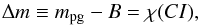 (1)where
χ(CI) is a function of the color index
CI. If only one color index (e.g.
(B − V)) is linearly involved in the color Eq. (1), we
may simplify this equation to
(1)where
χ(CI) is a function of the color index
CI. If only one color index (e.g.
(B − V)) is linearly involved in the color Eq. (1), we
may simplify this equation to  (2)The constant C
is called the color term. The value of the constant K may be
determined by the demand Δm = 0 for a specific subclass of objects. We
add the following notes to clarify the concept of photographic magnitude.
(2)The constant C
is called the color term. The value of the constant K may be
determined by the demand Δm = 0 for a specific subclass of objects. We
add the following notes to clarify the concept of photographic magnitude.
-
The notion of the photographic magnitude m pg, as we use it in thistext, generally applies to any magnitude determined from thephotographic plates, with no assumptions on the telescope,emulsion, or filter used. Moreover, atmospheric conditions may also vary within different plates. Therefore, the colorEq. (1) is a function of all these parameters, i.e.,the lens, filter, emulsion, atmospheric airmass, etc., and itmay take a different form for different sets of theseparameters.
-
Photographic magnitudes may be determined in different ways : by photographic density measurements, by disk-diameter measurements, or just by visual perception of the brightness (as in our case). The photographic plate is a nonlinear detector, i.e., the quantities (density, disk diameters, perceived brightness, etc.) through which we measure the magnitude of the object may exhibit a nonlinear dependence upon magnitude. Appropriate corrections have to be applied to handle this nonlinearity, alternatively a range of magnitudes with a linear response has to be used.
There are several ways to find the color Eq. (1):
-
A purely empirical approach fits the difference Δm between the photographic mpg and standard B magnitude against the color of the object to find the parameterization and color terms of the function χ(CI).
-
A theoretical reasoning gives the following equation for the difference Δm (Straizys 1963):
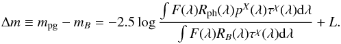 (3) In
Eq. (3) F(λ) is the
dereddened flux from the source,
Rph(λ) and
RB(λ)
are the response function of the two photometric systems,
pX(λ)
is the transmittance function of the atmosphere at X
air masses and
τx(λ)
is the transmittance function of the interstellar dust of
x unit masses. The
Rph(λ) response function
may be rewritten as
(3) In
Eq. (3) F(λ) is the
dereddened flux from the source,
Rph(λ) and
RB(λ)
are the response function of the two photometric systems,
pX(λ)
is the transmittance function of the atmosphere at X
air masses and
τx(λ)
is the transmittance function of the interstellar dust of
x unit masses. The
Rph(λ) response function
may be rewritten as 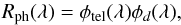 (4) where
φtel stands for the
transmittance function of the telescope (the lens plus filter) and
φd for the spectral
sensitivity of the photographic plate/emulsion. The spectral
sensitivity of the emulsion represents the dependence
of the quantity through which we measure the photographic magnitude upon
wavelength (i.e., photographic density, diameters of the disks, perceived
brightness, etc.). The
RB(λ)
response function is the standard B bandpass
response function (e.g. Bessel 1990). The constant L
in Eq. (3) may be determined by requiring
Δm = 0 for a specific subclass of objects (e.g. A0V
stars). Afterward, the synthetic photometry approach is applied: objects with
different spectra
(F(λ)) are the input
to the integrals of Eq. (3). The magnitude Δm
difference is fitted against theoretically computed standard color indices.
(4) where
φtel stands for the
transmittance function of the telescope (the lens plus filter) and
φd for the spectral
sensitivity of the photographic plate/emulsion. The spectral
sensitivity of the emulsion represents the dependence
of the quantity through which we measure the photographic magnitude upon
wavelength (i.e., photographic density, diameters of the disks, perceived
brightness, etc.). The
RB(λ)
response function is the standard B bandpass
response function (e.g. Bessel 1990). The constant L
in Eq. (3) may be determined by requiring
Δm = 0 for a specific subclass of objects (e.g. A0V
stars). Afterward, the synthetic photometry approach is applied: objects with
different spectra
(F(λ)) are the input
to the integrals of Eq. (3). The magnitude Δm
difference is fitted against theoretically computed standard color indices.
2.2.1. Magnitudes from photographic density measurements
Several authors have tried to find the color equations for different photographic
systems defined by different types of emulsions and telescopes with photographic
magnitude determined through photographic density measurements. We
briefly review at least some of the results. Generally, the
χ(CI) function of Eq. (1) is a function of several
color indices. Assuming only the (B − V) color index,
the color Eq. (1) for stars is nonlinear in this color index because
the Balmer jump is included in the photographic system (e.g. Arp 1961; Straizhis 1963). Arp
(1961) founds the best linear
fit for stars using only the (B − V) color
index (i.e., Eq. (1)) with a semi-empirical approach. The 103a-O
plates, aluminized reflector, and WG2 or GG1 filter are assumed as well. The resulting
color equation is  (5)For small
refractors that are free of chromatic aberration and Agfa plates and stars (not reddened
by dust) with color indices in the range
0.0 < (B − V)0 < 0.45,
Straizhis (1963) found with a theoretical
approach a similar color term (i.e., 0.18) to the equation of Arp
(1961). The equation of Arp (1961) has also been used in several papers to convert
photographic magnitudes to the standard B system (e.g. Schaefer et al. 1995; Hamuy et al. 1991), even though the emulsions and the telescope were different than in
Arp’s assumptions. Schaefer et al. (1995) argued
that the color terms for Harvard plates are expected to be close to zero.
(5)For small
refractors that are free of chromatic aberration and Agfa plates and stars (not reddened
by dust) with color indices in the range
0.0 < (B − V)0 < 0.45,
Straizhis (1963) found with a theoretical
approach a similar color term (i.e., 0.18) to the equation of Arp
(1961). The equation of Arp (1961) has also been used in several papers to convert
photographic magnitudes to the standard B system (e.g. Schaefer et al. 1995; Hamuy et al. 1991), even though the emulsions and the telescope were different than in
Arp’s assumptions. Schaefer et al. (1995) argued
that the color terms for Harvard plates are expected to be close to zero.
2.2.2. Isophotal magnitudes from digitized photographic plates
The color equation that relates the GSC2.2 B magnitudes and the magnitudes determined by the isophotal photometry from digitized Harvard plates results in a color term (for the GSC2.2 (B − R) color index) close to 0.2 for a wide range of Harvard plates and a wide range of series. The deviations of the color term from the mean value (0.2) seem to be fairly random in nature (for more details see Shaw et al. 2007).
2.2.3. Modified Argelander method
In case of the visual estimation of magnitudes, the photographic magnitudes are determined from the visual perception of the star diameters and the visual perception of their densities. Therefore, the color equation is generally different from those determined for photographic densities (by densitometers) or digitized photographic plates. First, we describe how we estimated the photographic magnitudes with the naked eye – the modified Argelander method. The method is still in use because it is fast and can be easily applied on original data material (i.e., glass photographic plates) without scanning. We note that many astronomical plate archives are not yet digitized, and the scanning of a large (typically many hundreds to many thousands) number of plates performed just for one particular object of interest would in many cases require huge efforts both in manpower and in time. Moreover, there are no scanners available in many plate archives.
The original Argelander method is used to visually estimate the brightness of stars in the sky (Schiller 1923; Hoffmeister 1984). We now describe the modification of this method, this time applied to the visual estimation of magnitudes on photographic plates. The disk of the estimated object on the plate is visually compared to the disks of nearby constant comparison stars of known B and V magnitudes. This visual comparison mainly relies on the perceived diameters of the disks, and partially on their perceived photographic density.
The approach of the modified Argelander method is as follows: On a specific plate, the perceived brightness of the studied object of interest (O) (star, blazar, etc.) is compared to the perceived brightness of (usually) two comparison objects (stars). One comparison star, Y, is brighter than the object O while the second comparison star, Z, is fainter. We denote with BY, BZ, and BO the standard B magnitudes of the comparison stars Y, Z, and the object O.
At first, the perceived brightness of the object O on the photographic plate is compared to the perceived brightness of the comparison star Y and an integer number of p Argelander steps is assigned to the perceived difference. Argelander steps are an observer-dependent (subjective) unit. The higher the number of Argelander steps, the higher the perceived difference in the brightness of the stars, and vice versa. Zero Argelander steps correspond to the case when the perceived brightness of the object and the perceived brightness of the comparison star are equal. Secondly, the perceived brightness of the object O is compared to the perceived brightness of the comparison star Z, and q Argelander steps are assigned to the perceived difference. This process results in the common notation YpOqZ and is repeated for other plates possibly using different comparison stars.
Assigning zero Argelander steps to the comparison star Y, p Argelander steps to the object O, and p + q Argelander steps to the comparison star Z, we obtain the brightness of the objects expressed in the Argelander scale. Because the comparison stars Y and Z are close in their brightness, we may assume that this scale is linearly proportional to the standard B magnitude scale, up to a color correction, i.e., we may write the following color equations (see Eq. (1) – we use different subscripts to denote potentially different functions χ(CI) for objects O, Y and Z)
![Mathematical equation: \begin{eqnarray} &&O = \alpha [B_{\rm Y} + \chi_{\rm Y} (CI_{\rm Y})] + \beta \\[2mm] &&p = \alpha [B_{\rm O} + \chi_{\rm O} (CI_{\rm O})] + \beta \\[2mm] &&p + q = \alpha [B_{\rm Z} + \chi_{\rm Z} (CI_{\rm Z})] + \beta , \end{eqnarray}](/articles/aa/full_html/2013/11/aa19323-12/aa19323-12-eq32.png) where
α and β denote the constants of the linear relation.
From this set of equations, it follows that
where
α and β denote the constants of the linear relation.
From this set of equations, it follows that ![Mathematical equation: \begin{eqnarray} &&B_{\rm O} = \frac {pB_{\rm Z} + qB_{\rm Y}}{p + q} + \psi \\[2mm] &&\psi \equiv \frac {p(\chi_{\rm Z}(CI_{\rm Z}) - \chi_{\rm O}(CI_{\rm O}) + q(\chi_{\rm Y}(CI_{\rm Y}) - \chi_{\rm O}(CI_{\rm O}))}{p + q}\cdot \end{eqnarray}](/articles/aa/full_html/2013/11/aa19323-12/aa19323-12-eq33.png)
The estimate of the BO magnitude is the interpolation of the BY and BZ magnitudes plus a color-correction term ψ, which involves the colors of all three objects. The assumption of the linear relation between Argelander scale and the standard B magnitude scale, up to a color correction, is justified within a limited small range of magnitudes.
Generally, χO, χY, χZ of Eqs. (6)–(8) are different functions for different plates, even if the objects O, Y, and Z are the same. This is because different plates were taken under different atmospheric conditions and with telescopes (objective, filter, and emulsion) with a different spectral response. After calibration, the Argelander steps can be transferred to the magnitude scale. For an experienced observer, the value of one step is always less than 0.1 mag and most typically between 0.06 and 0.08 mag.
3. Measurements II: HCO results
In our case, the studied object O is the blazar OJ 287 and the comparison stars Y and Z are pairs of stars of Table 1. The Harvard plates were taken with different telescopes and with different emulsions under different atmospheric conditions. Unfortunately, the information about the telescopes and emulsions used and their characteristics and changes is rarely available for Harvard plates (priv. comm. with A. Doane – plate stacks curator).
The accuracy of our measurements is not expected to be better than 0.1 mag, because we deal mostly with sky patrol plates (and hence not very deep limiting magnitudes). With this expectation we can accommodate the following assumptions:
-
We assume that all blue Harvard plates have one com-mon spectral response, even though they were taken withdifferent telescopes, emulsions, and under different at-mospheric conditions. This assumption may be justifiedby the results of Schaefer et al. (1995) andShaw et al. (2007), which show that the colorterms (in the color equations for density measurementsand in the color equation for isophotal photometry withdigitized plates) are approximately the same for different Harvard blue plates and series. We calculated the atmo-spheric airmass for all observations and evaluated onlythose estimates taken on plates within the range of air massesfrom 1 < X < 1.5. By excluding plates with higher air masses than this range, we prevent any additional enhancement of the difference in the spectral response of different plates.
-
Generally, χO or χY or χZ of Eqs. (6), (7) and (8) are nonlinear functions of color indices CIO or CIY or CIZ. We assume only a linear function in the (B − V) color index, i.e.,
 (11)
(11)![Mathematical equation: \begin{eqnarray} &&\nonumber\\[-12mm] &&\chi_{\rm Y}(CI_{\rm Y}) = C_{\rm Y}(B-V)_{\rm Y} + K_{\rm Y} \\[2mm] &&\chi_{\rm Z}(CI_{\rm Z}) = C_{\rm Z}(B-V)_{\rm Z} + K_{\rm Z}. \end{eqnarray}](/articles/aa/full_html/2013/11/aa19323-12/aa19323-12-eq45.png) This
approach of only one color linearly involved in the color equation is very common
for the photographic magnitude to the standard B
magnitude transformations.
This
approach of only one color linearly involved in the color equation is very common
for the photographic magnitude to the standard B
magnitude transformations. -
Because Y and Z are stars, we may assume that CS ≡ CY = CZ and KS ≡ KY = KZ, which leads to the following set of equations
![Mathematical equation: \begin{eqnarray} &&\chi_{\rm O}(CI_{\rm O}) = C_{\rm O}(B-V)_{\rm O} + K_{\rm O} \\[1mm] &&\chi_{\rm Y}(CI_{\rm Y}) = C_{\rm S}(B-V)_{\rm Y} + K_{\rm S} \\[1mm] &&\chi_{\rm Z}(CI_{\rm Z}) = C_{\rm S}(B-V)_{\rm Z} + K_{\rm S}. \end{eqnarray}](/articles/aa/full_html/2013/11/aa19323-12/aa19323-12-eq48.png) The
existence of one color term CS
common to all stars of different colors is justified by the results of
Schaefer (1995),
Arp (1961), Shaw
(2007), etc., which
suggest a single color term is applicable to stars of different spectra. With this
assumption the estimate of BO
magnitude may be rewritten as
The
existence of one color term CS
common to all stars of different colors is justified by the results of
Schaefer (1995),
Arp (1961), Shaw
(2007), etc., which
suggest a single color term is applicable to stars of different spectra. With this
assumption the estimate of BO
magnitude may be rewritten as
![Mathematical equation: \begin{eqnarray} &&B_{\rm O} = \frac {pB_{\rm Z} + qB_{\rm Y}}{p + q} + \psi \\[1mm] &&\psi = \frac {p[C_{\rm S}(B-V)_{\rm Z} - C_{\rm O}(B-V)_{\rm O} + K_{\rm S} - K_{\rm O}]}{p + q}\nonumber\\[1mm] && \qquad+~ \frac { q[C_{\rm S}(B-V)_{\rm Y} - C_{\rm O}(B-V)_{\rm O} + K_{\rm S} - K_{\rm O}]}{p + q}\cdot \end{eqnarray}](/articles/aa/full_html/2013/11/aa19323-12/aa19323-12-eq50.png)
3.1. Determining the color term CS for stars
To determine CS (i.e., the color term for stars), we estimate the brightness of stars of known B and V magnitudes. This means O is a star (of known magnitude) in the estimate YpOqZ, which implies CS ≡ CO = CY = CZ and KS ≡ KO = KY = KZ. With these assumptions the estimate of BO may be written as
![Mathematical equation: \begin{eqnarray} &&B_{\rm O} = \frac {pB_{\rm Z} + qB_{\rm Y}}{p + q} + \psi \quad\quad\\ &&\psi = C_{\rm S} \frac {p[(B-V)_{\rm Z} \! - \!(B-V)_{\rm O}] \!+\! q[(B-V)_{\rm Y} - (B-V)_{\rm O}]}{p + q}\cdot\quad\quad \end{eqnarray}](/articles/aa/full_html/2013/11/aa19323-12/aa19323-12-eq55.png) We
see that the constants KS have canceled out in Eq. (18).
Because we know the magnitude BO and
VO beforehand, the color term CS
may be determined by fitting
We
see that the constants KS have canceled out in Eq. (18).
Because we know the magnitude BO and
VO beforehand, the color term CS
may be determined by fitting 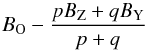 (21)versus
![Mathematical equation: \begin{equation} \psi = C_{\rm S} \frac {p[(B-V)_{\rm Z} \! -\! (B-V)_{\rm O}] \! +\! q[(B-V)_{\rm Y} \! -\! (B-V)_{\rm O}]}{p \! +\! q}\cdot \end{equation}](/articles/aa/full_html/2013/11/aa19323-12/aa19323-12-eq59.png) (22)To find
CS we estimated the magnitudes of more than 20 constant
stars of different colors in the field of the OJ 287 blazar as well as in the field of
other blazars – blazars, which we measured during our stay at Harvard. The magnitude of an
individual star was estimated several times on different plates. The values of
CS of different plates differ, with the average
CS ≈ 0.6. The estimate of 1–sigma error
ΔCS in the estimation of the mean value of
CS is ΔCS ≈ 0.2.
(22)To find
CS we estimated the magnitudes of more than 20 constant
stars of different colors in the field of the OJ 287 blazar as well as in the field of
other blazars – blazars, which we measured during our stay at Harvard. The magnitude of an
individual star was estimated several times on different plates. The values of
CS of different plates differ, with the average
CS ≈ 0.6. The estimate of 1–sigma error
ΔCS in the estimation of the mean value of
CS is ΔCS ≈ 0.2.
Calculating the B magnitudes of stars according to Eq. (19) with the color term CS = 0.6, we may determine the root mean square error Δmag in the estimation of B magnitudes of constant stars with the modified Argelander method. We have found the following
Δmag ≈ 0.15, for BZ − BY ≤ 0.75 mag
Δmag ≈ 0.20, for 0.75 mag < BZ − BY ≤ 1.50 mag
Δmag ≈ 0.30, for 1.50 mag < BZ − BY ≤ 2.50 mag
Δmag ≈ 0.40, for BZ − BY > 2.50 mag.
We see that the error increases as the magnitude separation of the two comparison stars increases. To achieve an acceptable (i.e. ≤0.2 mag) 1-sigma error, comparison stars have to be close in their brightness (i.e. BZ − BY < 1.5 mag).
3.2. Determining the color correction for OJ287
The color term CO for blazars is generally different from the color term CS for stars, and so is the additive constant KO different from the additive constant KS (see Eqs. (14), (15), and (16)). This is because stars and blazars have a different spectral energy distribution from stars in the optical region. The optical spectrum of OJ 287 exhibits only weak spectral lines (e.g. Sitko & Junkkarinen 1985; Stickel et al. 1989; Nilsson et al. 2010). Fν of OJ 287 exhibits a power–law profile Fν ~ ν−α in the optical region, with dereddened average α = 1.59 ± 0.22 (Fiorucci 2004). The spectrum of OJ 287 is also variable in the optical region.
The B magnitude of OJ 287 is estimated using Eq. (17). The correction
term (18) may be rewritten as ![Mathematical equation: \begin{eqnarray} \psi &=& \frac {p[C_{\rm S}(B-V)_{\rm Z}] + q[C_{\rm S}(B-V)_{\rm Y}]}{p + q} \nonumber \\[2mm] &&- [C_{\rm O}(B-V)_{\rm O} - K_{\rm S} + K_{\rm O}]. \end{eqnarray}](/articles/aa/full_html/2013/11/aa19323-12/aa19323-12-eq80.png) (23)The
value of the first fraction in the correction (23) is known because we know the color term
CS and the color indices of comparison stars Y and Z. The
second term, i.e.,
(23)The
value of the first fraction in the correction (23) is known because we know the color term
CS and the color indices of comparison stars Y and Z. The
second term, i.e., ![Mathematical equation: \begin{equation} - [C_{\rm O}(B-V)_{\rm O} - K_{\rm S} + K_{\rm O}] \end{equation}](/articles/aa/full_html/2013/11/aa19323-12/aa19323-12-eq81.png) (24)may be considered as an
additional color correction for OJ287 and may be determined by an
empirical approach. This consists of comparing estimates of magnitudes from plates with
known magnitudes of OJ 287 of the same date as the date of the plate exposure. This is
possible because the sampling of the previously known light curve of OJ 287 is quite
dense, therefore several previously known magnitudes overlap in time with the dates of
measurements from plates. For this purpose, we used the OJ287 database presented by
Valtonen et al. (2006), excluding suspicious
points.
(24)may be considered as an
additional color correction for OJ287 and may be determined by an
empirical approach. This consists of comparing estimates of magnitudes from plates with
known magnitudes of OJ 287 of the same date as the date of the plate exposure. This is
possible because the sampling of the previously known light curve of OJ 287 is quite
dense, therefore several previously known magnitudes overlap in time with the dates of
measurements from plates. For this purpose, we used the OJ287 database presented by
Valtonen et al. (2006), excluding suspicious
points.
We have to be aware of two important problems with this approach:
-
The color of OJ 287 exhibits temporal changes (e.g. Takalo &Sillanpää 1989; Fiorucci et al. 2004). Takalo &Sillanpää (1989) claimed that B − V was higher when OJ 287 was fainter during the years after 1971. We used the data of the OJ 94 project (Pursimo et al. 2000) and fitted the B − V color index versus the V magnitude. We found no significant correlation between the B − V color index and the V magnitude in the period of the OJ 94 project (i.e., 1993–1997) and have found the average B − V to be 0.45. Because the modified Argelander method is only an one-band photometrical approach, we are not able to evaluate the color of OJ287 at the moment of the measurement on the plate. Because there is no clear way how to determine the value of B − V for the measurement on the plate (e.g., determine it from OJ287 brightness), we are left with evaluating the color correction assuming a constant color index (B − V) = 0.45.
-
Even with excluding suspicious data from the previously known light curve, the magnitudes of OJ287 of this light curve are not determined accurately (i.e., they still have an error). If we assume that these magnitudes are unbiased estimates of the true magnitudes, then involving several data points gives an unbiased estimate of the color correction (23) for OJ 287, with a relatively small error.
Our results show that ![Mathematical equation: \begin{equation} - [C_{\rm O}(B-V)_{\rm O} - K_{\rm S} + K_{\rm O}] \approx 0.1. \end{equation}](/articles/aa/full_html/2013/11/aa19323-12/aa19323-12-eq85.png) (25)The correction term
for OJ 287 is close to 0.1, which means that OJ 287 results in a similar photographic
perception as the perception of a star with the B − V
index equal to −0.2. Furthermore we found the following root mean square errors Δmag in
determining the magnitude of OJ287: Δmag ≈ 0.3 mag. This result suggests that the
magnitudes of OJ 287 obtained from regular sky-survey photographic plates are not very
accurate, but still may provide valuable information if they are the only magnitudes in a
sparsely sampled epoch, and the amplitudes of light variations investigated are large
(>0.8 mag).
(25)The correction term
for OJ 287 is close to 0.1, which means that OJ 287 results in a similar photographic
perception as the perception of a star with the B − V
index equal to −0.2. Furthermore we found the following root mean square errors Δmag in
determining the magnitude of OJ287: Δmag ≈ 0.3 mag. This result suggests that the
magnitudes of OJ 287 obtained from regular sky-survey photographic plates are not very
accurate, but still may provide valuable information if they are the only magnitudes in a
sparsely sampled epoch, and the amplitudes of light variations investigated are large
(>0.8 mag).
New observational results for OJ287 from measurements on HCO plates.
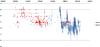 |
Fig. 1 Long-term (>100 years) B-mag light curve (B-magnitude versus year) of OJ287 based on data referenced by Takalo (1994). The newly added photometric points reported in this paper, as well as unpublished photographic measurements by Rene Hudec from the Sonneberg Observatory archival plates are marked by red squares. |
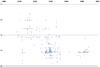 |
Fig. 2 New measurements (B-mag) of OJ287 from the HCO sky patrol plates reported in this paper plotted as light curve B-mag versus year. |
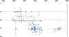 |
Fig. 3 New photometric points (circles) of OJ287 from new HCO measurements, with upper limits indicated (for the dates when the object was fainter than the relevant plate magnitude limit, red squares), plotted as light curve B-mag vs. year. For these new magnitude estimates the survey HCO plates (not used for OJ287 before) with lower plate limits than field plates (of higher quality but less numerous) were used. These results confirm that even the survey archival photographic plates with target magnitude near the plate limits can provide scientifically valuable results (note that for the dates of these points there are no other measurements available). |
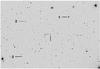 |
Fig. 4 Comparison stars used for estimating the brightness of OJ287 around the year 1913 (Digital Sky Survey map). OJ287 is also marked in the center of the image. The FOV of the plotted area is approximately 20 arcmin × 30 arcmin, north is top and east to the left. |
We give the results of our measurements in Table 2. For each Julian Day (JD), there is an estimate of the plate quality (Col. 2), the B magnitude (Col. 3), and letter u if the measurement refers to an upper limit. Actual measured values have no letter in this column (Col. 4). Only the first few historical measurements are given here, the full table is available at the CDS. In Fig. 1 we add the new measurements to the old light curve, and find that the new points enforce the earlier impression of an outbursts at approximately 12 year cycles. The same cyclic behavior is seen in the new measurements on their own (Fig. 2); including upper limits does change this impression (Fig. 3). The upper limits can be used to exclude the possibility of outbursts at certain times, and they thus also provide useful information. We discuss below how the upper limits of the spring 1906 constrain the binary black hole model of OJ287. Figure 4 shows that OJ287 is easily detected when it is in its bright state; similarly the non-detection of OJ287 often indicates that OJ287 is in a low state, not in an outburst.
In total, we obtained 573 new data points for OJ287 from the HCO plate analyses (364 measurements and 209 upper limits).
4. Discussion
4.1. The 1913 flare
We now discuss some parts of the measured light curve that are of special interest. Starting with the 1913 major outburst, in Table 3 we present the newly measured data to the OJ 287 light curve. The estimated errors are based on the results above plus the quality of the plate. In Table 4 we summarize the earlier data referenced by Takalo (1994). The combined data are plotted in Fig. 5.
New measurements of OJ287 for the 1913 flare (this paper).
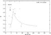 |
Fig. 5 Light curve of the 1913 flare in OJ287. The B-band light curve combines old (stars) and new (squares) measurements. The theoretical light curve of about 46-day duration at half-maximum is also shown. The starting point of the outburst is at about 1912.96 in this fit. The three small arrows indicate the positions of the three possible flares mentioned in the text. |
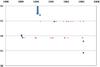 |
Fig. 6 Light curve (B-mag versus year) of the 1900 OJ287 flare, reported for the first time. The circles represent measurements, the triangles represent the upper limits, both for HCO sky survey plates. The position of the calculated outburst is indicated by an arrow. |
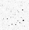 |
Fig. 7 OJ287 near the 1913 maximum on a scanned HCO sky-survey photographic plate. The FOV of the area plotted is approximately 40 arcmin × 40 arcmin, north is top and east is to the left, and the comparison stars from Table 1 are indicated (star 3 is just at the plate threshold). |
In Fig. 7 we present the scan of the JD = 2 419 780.784 plate, i.e., plate taken around the maximum of the 1913 outburst. Valtonen et al. (2010) discussed the observations of the 1913 outburst in OJ287 and how they can be used in the precessing binary black hole model. The expected length (at half-maximum) of the 1913 outburst in the model of Lehto & Valtonen (1996) is 0.126 yr or 46 days. Figure 5 shows that this is more or less correct, i.e., the model prediction and the observations agree. The beginning of the flare is at 1912.96. It agrees within error limits of 0.02 yr with the value used in earlier papers (Valtonen et al. 2010, 2011b). The estimate of the flare start is based on the standard flare profile (Valtonen et al. 2011b) overlaid with observations. The errors in individual observations as well as flaring in the source complicate the fit. The large sampling gaps also prevent a precise timing of the flare.
There is some flaring in addition to the standard outburst light curve, as is observed in other similar outbursts (Valtonen et al. 2008). The three flares indicated in Fig. 5 are separated by approximately 50 days, the half-period of the innermost stable orbit of the primary black hole. We note that the HCO plate data are consistent with the three flares, but they are not not good enough to confirm these flares. The same flaring frequency has been seen in recent times in longer observational sequences (Valtonen et al. 2011a).
4.2. The 1900 flare
This outburst of OJ 287 is newly discovered, i.e., it was unknown before, and represents the oldest outburst of this object ever detected. It occurred at JD 2 415 119.627, i.e., 1900.27, when the object reached B magnitude 12.61, i.e., V magnitude 12.16, the brightest magnitude in 50 years. The relevant HCO plate is of a very good quality. The object was studied in detail by high magnifying microscopy to ensure that this is a real image.
4.3. Historical 1900 and 1913 outbursts from the point of view of the binary black hole model
In the binary black hole model of Lehto & Valtonen (1996) and Sundelius et al. (1997) there are two main sources of optical outbursts. The first kind arises when the secondary black hole impacts on the accretion disk of the primary, and extracts a hot gas cloud (Ivanov et al. 1998). Radiation from this cloud is Bremsstrahlung radiation. The total flux is low as long as the cloud is optically thick. When the cloud becomes optically thin, the flux suddently increases on the time scale of the light travel time through the cloud. Subsequently, the energy density in the cloud decreases because of its expansion, and the flux decreases as −(3/2) power of time. The impacts at different times take place at different distances from the primary black hole. The flux-decrease time scale becomes longer with the increasing distance between the impact site and the primary black hole.
To simulate the dynamics of the OJ287 system, we developed a multiprocessor N-body solver, along the lines of the model of Sundelius et al. (1997), but with significant improvements. The orbits of the black hole binary and the accretion disk of the primary are calculated simultaneously, and the mutual interactions between the accretion disk particles are taken into account, unlike in the Sundelius et al. (1977) calculation.
The accretion disk is modeled as a cloud of point particles initialized with a standard vertical sech2(z/z0) distribution, where z is the vertical height in the disk, and z0 is the scale height. The point particles interact gravitationally both with black holes of the binary and with each other through a grid-based viscosity calculation.
For the disk viscosity calculation we used a radially nonuniform polar grid adapted from Miller (1976). In this scheme the grid cells are approximately square through the entire radial extent of the grid. The disk viscosity is calculated in the vertical direction only, using the physical model of Lehto & Valtonen (1996) to obtain the kinematic viscosity coefficient as a function of the radial distance.
Additionally, the solver uses the post-Newtonian approximation scheme to calculate the gravitational interaction of the black hole binary and the forces between the primary black hole and the accretion disk particles. Post-Newtonian terms up to and including order 3 were used.
We illustrate the result of one such simulation in Fig. 8. The orbit is not a closed ellipse but precesses in a forward sense. It is easy to see why a closed orbit without precession does not work. Take the two prominent outbursts in 1913 and in 1983. The six cycles between 1913 and 1983 have an average interval of 11.665 yr. However, this constant interval is not observed. For example, the outburst that is projected to 2006.33 by the average interval actually happened at 2005.76 (Valtonen et al. 2008). In the same way, an outburst projected at 1901.33 actually took place in 1900.27, as we saw above. This is the typical discrepancy between the projections and the actual observed outburst times in a constant-period model.
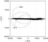 |
Fig. 8 Orbit of the secondary around the primary, which is approximately at the point (0,0). The coordinate units are given in AU. The disk is seen edge-on. The secondary orbits the primary in a counter-clockwise sense. The last point in the orbit is in the year 1915; the previous disk crossings occurred in 1912 and 1910. The disk crossing farthest to the left happened in 1903, and previous crossings were in 1898 and 1895. Because of precession the intervals between disk crossings vary greatly. |
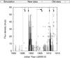 |
Fig. 9 Accretion rate in the precessing binary black hole model (vertical lines) compared with the observed brightness of OJ287 (squares: data from this paper, circles: previously published data) in linear scale. The vertical arrows mark the expected times of outbursts arising from the disk crossings by the secondary, while the horizontal arrows indicate the time delays between the disk impacts and the related outbursts. |
The second source for optical outbursts is the tidal transfer of disk matter toward the central black hole where some of the matter is transferred into a jet. The synchrotron radiation from the jet is observed at all times, but there is a periodic enhancement of the radiation when the accretion rate of matter is at its highest. It happens when the secondary comes close to the primary black hole. Figure 9 illustrates the expected tidal accretion rates between 1890 and 1915 and compares them with the observed brightness of OJ287. We notice that the brightest observed magnitude in 1900 coincides with the highest accretion peak in the same year. The high level of activity in OJ287 in 1911 is also apparently generated by a high accretion rate.
These peaks are also seen in the simulation by Sundelius et al. (1997), which is based on the orbit model of Lehto & Valtonen (1996). Because of the different precession rate of the Lehto & Valtonen (1996) model and the present model, the direction of the main axis of the binary orbit is quite different in these two models in 1900. Consequently, the accretion rate as calculated by Sundelius et al. (1997) peaked a year earlier that in our calculation. The agreement of the present model with observations is additional evidence that the new orbit solution by Valtonen (2007) with a 39-degree precession rate per period is superior to the old solution by Lehto & Valtonen (1996), which had a 33-degree precession rate per period.
There are no observations to check the precessing binary model for the late-1800 disk crossings. The outburst related to the 1903 disk crossing should start in the interval 1906.15–1906.25, lasting about 0.15 yr (the exact value depends on the primary spin). There is a gap in the new measurements, but we have several interesting upper limits in the spring of 1906 (see also Fig. 3): 1906.06 (B > 14.1), 1906.08 (B > 13.0), 1906.13 (B > 14.1), 1906.15 (B > 14.1), 1906.17 (B > 13.0), 1906.24 (B > 13.0, bad plate), 1906.31 (B > 14.1) and 1906.37 (B > 13.0). The only gap of sufficient length to contain an outburst of the expected size and duration is between 1906.15 and 1906.31; if the outburst really happened, its starting time should be near the beginning of this gap, around 1906.15. This outburst time favors the normalized spin value around 0.23, which is at the lower end of the possible range determined previously (Valtonen et al. 2010). The observed peak at 1910 cannot be the direct result of the disk impact in that year, but it is more likely a “precursor” (Valtonen et al. 2006). Precursors first occur when the secondary approaches the primary disk at the level of about 20 disk scale heights. Prominent precursors were seen in 1993 and 2004 prior to the 1994 and 2005 primary outbursts; the corresponding precursor in 1910 should have been observed in the spring of that year. The actual outburst peak was expected during the following summer when OJ287 was not observable.
These results confirm the enormous scientific value of old records on astronomical plates. The recent findings of one of the authors of this paper (RH) that there are several additional major large plate collections with old records in the US, which are unknown to the astronomical community and with no access yet to their catalogs (Hudec & Hudec 2013), gives us hope that we may be able to find additional sources of historical data for OJ287 and other objects that require very old data. Even the European astronomical plate collections may still include so-far uncatalogued plates that are hidden from the astronomical community. This is confirmed by recent findings of one of authors (RH) of Göttingen Observatory plates taken in 1910–11 that are stored in the Bamberg Observatory archive.
5. Conclusion
The new observations of the historical records of OJ287 reveal for the first time the as yet unknown 1900 outburst. We identified it as an outburst that arose from an increased accretion rate when the two black holes were close to each other. According to our calculations, the rate should have peaked at just this time. We also saw for the first time the rising part of the 1913 outburst. It shows that the length of the outburst is as expected from the precessing binary model if it is related to a disk impact. We also found that the outburst started at around 1912.96. This timing is consistent with the latest orbit solution of OJ287 (Valtonen et al. 2010).
The mean period between 1913 and 1983 is 11.665 yr, assuming that six cycles fit inside this interval. If outbursts were repeated at this interval, there should have been one at 1948.00, while an outburst was seen at 1947.30; the next predicted outburst would have been at 1959.70, while the event was seen at 1959.23; and finally the predicted 2006.33 outburst was seen at 2005.76. Obviously, there is no strict periodicity in the optical outburst pattern of OJ287. With the precessing binary black hole model one can understand the systematics of outburst timings.
This study confirms the importance of archival astronomical plates in general and in analyses of blazars in particular. This is also justification for the recent efforts for data mining and the wide digitization of the world’s astronomical plate archives. There is in fact no other way to check the behavior of astrophysical objects over dozens of years and sometimes for even more than a century.
Acknowledgments
We acknowledge travel support provided by the Smithsonian Institution for our HCO stay as well as by GA CR, grants 102/09/0997 and 13-39464J. We thank V. Hudcová for help in preparing the figures and literature references for this paper.
References
- Agudo, I., Jorstad, S. G., Marscher, A. P., et al. 2011, ApJ, 726, L13 [NASA ADS] [CrossRef] [Google Scholar]
- Arnett, W. D. 1979, ApJ, 230, L37 [NASA ADS] [CrossRef] [Google Scholar]
- Arp, H. 1961, ApJ, 133, 869A [NASA ADS] [CrossRef] [Google Scholar]
- Bessel, M. S. 1990, PASP, 102, 1181 [NASA ADS] [CrossRef] [Google Scholar]
- Craine, E. R. 1977, A handbook of quasistellar and BL Lacertae objects, Astronomy and Astrophysics Series (Tucson: Pachart) [Google Scholar]
- Fiorucci, M., Ciprini, S., & Tosti, G. 2004, A&A, 419, 2534 [NASA ADS] [CrossRef] [EDP Sciences] [Google Scholar]
- Hamuy, M., Phillips, M., Maza, J., et al. 1991, AJ, 102, 208 [NASA ADS] [CrossRef] [Google Scholar]
- Hoffmeister, C. 1984, Veraenderliche Sterne (Leipzig: Johann Ambrosius Barth) [Google Scholar]
- Hudec, R. 1990, Acta Historica Astron., 6, 28 [Google Scholar]
- Hudec, R. 2006, in Virtual Observatory: Plate Content Digitization, Archive Mining and Image Sequence Processing, Astro workshop, Sofia, Bulgaria, 2005 Proc., 197 [Google Scholar]
- Hudec, R. 2007, in Exploring the Cosmic Frontier: Astrophysical Instruments for the 21st Century. ESO Astrophysics Symp., European Southern Observatory series, eds. A. P. Lobanov, J. A. Zensus, C. Cesarsky, & P. J. Diamond (Berlin, Heidelberg: Springer-Verlag), 79 [Google Scholar]
- Hudec, R. 2010, The Astronomer’s Telegram, 2619 [Google Scholar]
- Hudec, R. 2011, JApA, 32, 91 [NASA ADS] [Google Scholar]
- Hudec, R., & Basta, M. 2006, in Virtual Observatory: Plate Content Digitization, Archive Mining and Image Sequence Processing, Astro workshop, Sofia, Bulgaria, 2005 Proc., 189 [Google Scholar]
- Hudec, R., & Hudec, L. 2013, Acta Polytechnica, 53, 23 [Google Scholar]
- Hudec, R., & Wenzel, W. 1976, BAI Czechoslovakia, 27, 325 [Google Scholar]
- Hudec, R., Šimon, V., & Hudec, L. 2009, in Frontier Objects in Astrophysics and Particle Physics, Vulcano Workshop 2008, eds. F. Giovannelli, & G. Mannocchi, 65 [Google Scholar]
- Ivanov, P. B., Igumenschev, I. V., & Novikov, I. D. 1998, ApJ, 507, 131 [NASA ADS] [CrossRef] [Google Scholar]
- Kidger, M. R. 2000, AJ, 119, 2053 [NASA ADS] [CrossRef] [Google Scholar]
- Lehto, H. J., & Valtonen, M. J. 1996, ApJ, 460, 207 [NASA ADS] [CrossRef] [Google Scholar]
- Miller, R. H. 1976, J. Comput. Phys., 4, 400 [NASA ADS] [CrossRef] [Google Scholar]
- Nilsson, K., Takalo, L. O., Lehto, H. J., et al. 2010, A&A, 516, A60 [NASA ADS] [CrossRef] [EDP Sciences] [Google Scholar]
- Pierce, M., & Jacoby, G. 1995, AJ, 110, 2885 [NASA ADS] [CrossRef] [Google Scholar]
- Pursimo, T., Takalo, L. O., Sillanpää, A., et al. 2000, A&AS, 146, 141 [NASA ADS] [CrossRef] [EDP Sciences] [Google Scholar]
- Rampadarath, H., Valtonen, M. J., & Saunders, R. 2007, Proc. Conf. held 16–21 October, 2006 at Xi’an Jioatong University, Xi’an, China, eds. L. C. Ho, & J.-M. Wang, ASP Conf. Ser., 373, 243 [Google Scholar]
- Schaefer, B. E. 1995, ApJ, 447, L13 [NASA ADS] [CrossRef] [Google Scholar]
- Schiller, K. 1923, Einfuehrung in das Studium der Veraenderlichen Sterne (Leipzig: Verlag von Johann Ambrosius Barth) [Google Scholar]
- Sillanpää, A., Haarala, S., Valtonen, M. J., et al. 1988, ApJ, 325, 628 [NASA ADS] [CrossRef] [Google Scholar]
- Sillanpää, A., Takalo, L. O., Pursimo, T., et al. 1996, A&A, 305, L17 [NASA ADS] [Google Scholar]
- Sitko, M. L., & Junkkarinen, V. T. 1985, PASP, 97, 1158 [NASA ADS] [CrossRef] [Google Scholar]
- Shaw, M. S., Grindlay, J. E., & Laycock, S. 2007, BAAS, 38, 1125 [NASA ADS] [Google Scholar]
- Stickel, M., Fried, J. W., & Kuehr, H. 1989, A&AS, 80, 103 [NASA ADS] [Google Scholar]
- Straizhis, V. 1963, Astron. Zh., 40, 332 [NASA ADS] [Google Scholar]
- Sundelius, B., Wahde, H., Lehto, H. J., et al. 1997, ApJ, 484, 180 [NASA ADS] [CrossRef] [Google Scholar]
- Takalo, L. O. 1994, Vist. in Astron., 38, 77 [Google Scholar]
- Tsvetkov, M. K., Stavinschi, M., Tsvetkova, K. P., et al. 2000, Balt. Astron., 9, 613 [NASA ADS] [Google Scholar]
- Valtonen, M. J. 2007, ApJ, 659, 1074 [NASA ADS] [CrossRef] [Google Scholar]
- Valtonen, M. J., Lehto, H. J., Sillanpää, A., et al. 2006, ApJ, 646, 36 [NASA ADS] [CrossRef] [Google Scholar]
- Valtonen, M. J., Kidger, M. R., Lehto, H. J., & Poyner, G. 2008, A&A, 477, 407 [NASA ADS] [CrossRef] [EDP Sciences] [Google Scholar]
- Valtonen, M. J., Nilsson, K.,Villforth, C., et al. 2009, ApJ, 698, 781 [NASA ADS] [CrossRef] [Google Scholar]
- Valtonen, M. J., Mikkola, S., Merritt, D., et al. 2010, ApJ, 709, 725 [NASA ADS] [CrossRef] [Google Scholar]
- Valtonen, M. J., Lehto, H. J., Takalo, L. O., et al. 2011a, ApJ, 729, 33 [NASA ADS] [CrossRef] [Google Scholar]
- Valtonen, M. J., Mikkola, S., Lehto, H. J., et al. 2011b, ApJ, 742, 22 [NASA ADS] [CrossRef] [Google Scholar]
All Tables
Comparison stars used for estimating the brightness of OJ287 on HCO plates around the year 1913.
All Figures
|
Fig. 1 Long-term (>100 years) B-mag light curve (B-magnitude versus year) of OJ287 based on data referenced by Takalo (1994). The newly added photometric points reported in this paper, as well as unpublished photographic measurements by Rene Hudec from the Sonneberg Observatory archival plates are marked by red squares. |
| In the text | |
|
Fig. 2 New measurements (B-mag) of OJ287 from the HCO sky patrol plates reported in this paper plotted as light curve B-mag versus year. |
| In the text | |
|
Fig. 3 New photometric points (circles) of OJ287 from new HCO measurements, with upper limits indicated (for the dates when the object was fainter than the relevant plate magnitude limit, red squares), plotted as light curve B-mag vs. year. For these new magnitude estimates the survey HCO plates (not used for OJ287 before) with lower plate limits than field plates (of higher quality but less numerous) were used. These results confirm that even the survey archival photographic plates with target magnitude near the plate limits can provide scientifically valuable results (note that for the dates of these points there are no other measurements available). |
| In the text | |
|
Fig. 4 Comparison stars used for estimating the brightness of OJ287 around the year 1913 (Digital Sky Survey map). OJ287 is also marked in the center of the image. The FOV of the plotted area is approximately 20 arcmin × 30 arcmin, north is top and east to the left. |
| In the text | |
|
Fig. 5 Light curve of the 1913 flare in OJ287. The B-band light curve combines old (stars) and new (squares) measurements. The theoretical light curve of about 46-day duration at half-maximum is also shown. The starting point of the outburst is at about 1912.96 in this fit. The three small arrows indicate the positions of the three possible flares mentioned in the text. |
| In the text | |
|
Fig. 6 Light curve (B-mag versus year) of the 1900 OJ287 flare, reported for the first time. The circles represent measurements, the triangles represent the upper limits, both for HCO sky survey plates. The position of the calculated outburst is indicated by an arrow. |
| In the text | |
|
Fig. 7 OJ287 near the 1913 maximum on a scanned HCO sky-survey photographic plate. The FOV of the area plotted is approximately 40 arcmin × 40 arcmin, north is top and east is to the left, and the comparison stars from Table 1 are indicated (star 3 is just at the plate threshold). |
| In the text | |
|
Fig. 8 Orbit of the secondary around the primary, which is approximately at the point (0,0). The coordinate units are given in AU. The disk is seen edge-on. The secondary orbits the primary in a counter-clockwise sense. The last point in the orbit is in the year 1915; the previous disk crossings occurred in 1912 and 1910. The disk crossing farthest to the left happened in 1903, and previous crossings were in 1898 and 1895. Because of precession the intervals between disk crossings vary greatly. |
| In the text | |
|
Fig. 9 Accretion rate in the precessing binary black hole model (vertical lines) compared with the observed brightness of OJ287 (squares: data from this paper, circles: previously published data) in linear scale. The vertical arrows mark the expected times of outbursts arising from the disk crossings by the secondary, while the horizontal arrows indicate the time delays between the disk impacts and the related outbursts. |
| In the text | |
Current usage metrics show cumulative count of Article Views (full-text article views including HTML views, PDF and ePub downloads, according to the available data) and Abstracts Views on Vision4Press platform.
Data correspond to usage on the plateform after 2015. The current usage metrics is available 48-96 hours after online publication and is updated daily on week days.
Initial download of the metrics may take a while.