| Issue |
A&A
Volume 558, October 2013
|
|
|---|---|---|
| Article Number | A98 | |
| Number of page(s) | 10 | |
| Section | Catalogs and data | |
| DOI | https://doi.org/10.1051/0004-6361/201321995 | |
| Published online | 11 October 2013 | |
Homogenization in compiling ICRF combined catalogs
1
Dep. Matemáticas, IMAC, Universitat Jaume I,
12071
Castellón,
Spain
e-mail: marco@mat.uji.es; lopez@mat.uji.es
2
Dep. Matematica Aplicada, IUMPA, Universidad Politécnica de
Valencia, 46022
Valencia,
Spain
e-mail:
mjmartin@mat.upv.es
Received:
30
May
2013
Accepted:
6
August
2013
Context. The International Astronomical Union (IAU) recommendations regarding the International Celestial Reference Frame (ICRF) realizations require the construction of radio sources catalogs obtained using very-long-baseline interferometry (VLBI) methods. The improvement of these catalogs is a necessary procedure for the further densification of the ICRF over the celestial sphere.
Aims. The different positions obtained from several catalogs using common sources to the ICRF make it necessary to critically revise the different methods employed in improving the ICRF from several radio sources catalogs. In this sense, a revision of the analytical and the statistical methods is necessary in line with their advantages and disadvantages. We have a double goal: first, we propose an adequate treatment of the residual of several catalogs to obtain a homogeneous catalog; second, we attempt to discern whether a combined catalog is homogeneous.
Methods. We define homogeneity as applied to our problem in a dual sense: the first deals with the spatial distribution of the data over the celestial sphere. The second has a statistical meaning, as we consider that homogeneity exists when the residual between a given catalog and the ICRF behaves as a unimodal pure Gaussian. We use a nonparametrical method, which enables us to homogeneously extend the statistical properties of the residual over the entire sphere. This intermediate adjustment allows for subsequent computation of the coefficients for any parametrical adjustment model that has a higher accuracy and greater stability, and it prevents problems related with direct adjustments using the models. On the other hand, the homogeneity of the residuals in a catalog is tested using different weights. Our procedure also serves to propose the most suitable weights to maintain homogeneity in the final results. We perform a test using the ICRF-Ext2, JPL, and USNO quasar catalogs.
Results. We show that a combination of catalogs can only be homogeneous if we configure the weights carefully. In addition, we provide a procedure to detect inhomogeneities, which could introduce deformities, in these combined catalogs.
Conclusions. An inappropriate use of analytical adjustment methods provides erroneous results. Analogously, it is not possible to obtain homogeneous-combined catalogs unless we use the adequate weights.
Key words: astrometry / celestial mechanics / methods: data analysis
© ESO, 2013
1. Introduction
The International Celestial Reference Frame (ICRF; Ma 1998) was officially adopted to replace its predecessor, the FK5 Frame, as the realization of the International Celestial Reference System (ICRS; Arias 1995) at the 23th International Astronomical Union (IAU) General Assembly in 1997. Catalogs of radio source positions (RSC) derived from VLBI observations have been used by the IAU to establish the ICRF since 1998. The first realization of the ICRF, the ICRF1, consisted of 608 extragalactic radio sources and 294 candidate sources to make future improvements possible and 102 additional unstable sources.
Definitions of the ICRF are no longer related to the equinox or equator, but the IAU has recommended that the new reference frame should be consistent with the former FK5 system for the sake of continuity. The principal plane should be close to the mean equator at J2000.0 and the origin of right ascension should be close to the dynamical equinox at J2000.0. Feissel 1998 concluded that the final orientations of the ICRF axes were coincident with those of the FK5 J2000.0 system within the uncertainties of the latter catalog.
In 1999, the first extension of ICRF1, the ICRF-Ext1 (IERS 1999) was released with 59 new sources as candidate sources. The positions and errors of the ICRF1 defining sources remained unchanged. The second extension of the ICRF1, the ICRF-Ext2 (Fey et al. 2004), added 50 new sources, and the positions of ICRF candidates and other sources were revised. The positions of the 212 defining sources were kept the same as those obtained in the ICRF1. It should be pointed out that both ICRF1 extensions were similarly obtained to the first realization, as a result of analysis of the VLBI observations at a single analysis center. The orientations of the ICRF-Ext2 axes and their uncertainties, however, still remained at the same level as for the original ICRF1.
The second realization of the ICRF, the ICRF2 (Fey et al. 2009) has 3414 objects (295 defining) and presents some advantages with respect to the previous realizations of the ICRF. The sky distribution of radio sources is improved by 1383 sources in the southern hemisphere, and the source categorization is subject to a more rigorous criterion. Only 97 defining sources of the ICRF1 remain as ICRF2 defining sources, and 39 unstable sources, some of which were ICRF1 defining sources, are identified as requiring special handling with their positions treated as arc parameters in VLBI data analysis. Statistical information on the evolution of the realization of the ICRS is given in (Yu 2013).
We focus our interest in the ICRF-Ext2, which is widely used for astrometrical measurements; thus, its accuracy and stability should be assured. This requires continuous maintenance as time elapses. First, the ICRF-Ext2 needs to be more densely defined because it includes a total of 717 sources and has a largely non-uniform distribution over the sky. Second, the defining sources have to be monitored to verify whether they are still proper and stable to be used in a future realization of the ICRS.
With regard to the first question above, attempts were made to improve the accuracy of the celestial reference frame by constructing combined catalogs after the appearance of the first VLBI radio sources catalog. Different methods were used to obtain a combined RSC with (Arias et al. 1988) being the first of them, and others were proposed by Walter (1989a, 1989b) and Yatskiv (1990). In accordance with Sokolova (2007), appropriate use of individual catalogs with common sources provides an improvement of each individual catalog. Among the general aims regarding this subject, we can point out the comparative study between catalogs and ICRF defining sources by considering a rigid frame (only rotations), avoiding deformations, and considering the densification of the ICRF in a twofold sense: the increased amount of defining sources and the densification in its wider sense of the catalog.
In all Cat-ICRF comparison processes, we intend to separate the residuals into two components: systematic errors (signal) and random errors (noise). During the study process of each individual catalog and the subsequent process of obtaining a combined catalog, we may find some problems that could provide unsatisfactory results. To study systematic errors, a parametrical model is a common choice and then the least squares method is indiscriminately used to obtain the coefficients of the chosen model, either geometrical (rotation or rotation plus deformation) or analytical (spherical harmonics development of Fourier-Legendre, for instance). Related to this, it may be extremely important that:
-
a)
The nonhomogeneity in the spatial distribution since it causesfunctional orthogonality does not turn into algebraicalorthogonality in the discrete case. This problem is especiallyserious when we estimate high order harmonics.
-
b)
The mean quadratic error is the sum of the mean squared bias and the variance. An artificial decrease of the bias (If the information is biased, the model must consider this possibility) implies an increase in the variance, and this could introduce artificial and undesirable deformations.
For suitable treatment of these possible complications, we use a double meaning for the word “homogeneous”. A first meaning refers to the spatial distribution of the data. Another one is applied to the remaining “remainder” after the geometric adjustment of the Cat-ICRF residuals that must behave as a unimodal Gaussian distribution with null mean. A detailed study of the first sense was developed in our papers (Marco 2004a) for Hipparcos-FK5, (Marco 2004b) for Hipparcos-Tycho2 and (Martínez 2009) for the estimation of the Hipparcos-FK5 spin. All these works were carried out in the context of a complete adjustment between catalogs with many common stars. In our present case, there are differences in the number of reference positions, because we have defining sources with higher quality and the rest are common objects. In the case of few common sources, the previously mentioned problems are worse, and we must be especially careful if we want to obtain the aims proposed above.
Let us go back to the decomposition for every catalog of the residual in the signal with the random part that must be normally distributed. A combination of catalogs take us generally to a random part that consists of one Gaussian mixture, which indicates the origin of the different sources used in the compilation. This shows that a combined catalog is not generally homogeneous in the second sense given to the word.
As we establish later, there is a specific assignment of weights that provides a residual that is a pure Gaussian distribution after the adjustment. This problem itself is very difficult to study. We have been able to make use of several procedures, such as a Gauss-induced by least squares or search, using minimization of the distance, as in Sfikas (2005). We consider the result given by the (not necessarily the most efficient) method, where homogenization is (at least) assured in a radius equal to the standard deviation and is centered in the mean. This problem would not be complete if we do not provide an answer to the inverse problem: given a nonhomogeneously combined catalog, how can we find the different populations from which it originates? The answer is not evident. We respond to another problem that may answer the former one: given one Gaussian mixture, how could we obtain the summands in which it decomposes? This part deals with the study of the random component of the residuals. These two questions are considered in the following section. The presentation of the problem is covered in greater detail and more suitable terminology and answers are provided to both previous questions. In the Appendix, a rigorous proof is included regarding the convergence of methods in a more general case.
Concerning the previously mentioned decomposition of the mean-quadratic error in the mean-squared bias and the variance from a statistical point of view, several approaches to this problem exist. The usual one consists of minimizing empirical errors, choosing a parametrical adjustment model. In this case, the coefficients of the model are very susceptible to changes in the initial data, being sensitive to spatial distribution and to the individual errors that they contain. On the other hand, we propose an approach to the problem with better stability properties. It implies the use, as an intermediary, of a non parametrical adjustment. We see some additional advantages of using this approach, which is the aim of the third section. In the fourth section, we give a summary of the parametrical approach. In the fifth section, we consider all the previous considerations for the use of two quasar catalogs to improve the ICRF. This paper concludes with a brief summary of conclusions and a final Appendix.
2. Homogeneity and errors in combined catalogs
Let
{xi, i = 1, 2, ...n}
be the ICRF positions, and let  =
1, 2, ...n},
=
1, 2, ...n},
 be the
corresponding values in the two other catalogs. We work with the original positions
{ xi, i =
1, 2, ...n } and the
residuals
{yi, i = 1, 2, ...n}
and
{zi, i = 1, 2, ...n}
for Catalog1-ICRF or Catalog2-ICRF. Suppose that we have
be the
corresponding values in the two other catalogs. We work with the original positions
{ xi, i =
1, 2, ...n } and the
residuals
{yi, i = 1, 2, ...n}
and
{zi, i = 1, 2, ...n}
for Catalog1-ICRF or Catalog2-ICRF. Suppose that we have
![\begin{equation} y_{i}=m^{[1] }(x_{i})+\varepsilon _{i}^{[1] },z_{i}=m^{ [2] }(x_{i})+\varepsilon _{i}^{[2] }, \end{equation}](/articles/aa/full_html/2013/10/aa21995-13/aa21995-13-eq9.png) (1)where each
(1)where each
![\hbox{$\varepsilon _{i}^{[j] },j=1,2$}](/articles/aa/full_html/2013/10/aa21995-13/aa21995-13-eq10.png) is a normal random variable
with
is a normal random variable
with  ,
,
 respectively and
m[1],m[2]
models of adjustment. In general, any linear combination of random variables (RV henceforth)
is not a pure Gaussian, but a Gaussian mixture. In the particular case of being a pure
Gaussian, we say that we have a homogeneous combined catalog.
respectively and
m[1],m[2]
models of adjustment. In general, any linear combination of random variables (RV henceforth)
is not a pure Gaussian, but a Gaussian mixture. In the particular case of being a pure
Gaussian, we say that we have a homogeneous combined catalog.
Thus, we want to find a new RV U and a model m from the
RV Y,Z and the models
m[1],m[2] so
that the residual U − m(X) verifies that
it is a pure Gaussian RV with null expectation and that
 .
.
Taking ![\hbox{$m\left( X\right) =\alpha _{1}m^{[1] }\left( X\right) +\alpha _{2}m^{[2] }\left( X\right) $}](/articles/aa/full_html/2013/10/aa21995-13/aa21995-13-eq20.png) and
U = α1Y + α2Z,
it is evident that
and
U = α1Y + α2Z,
it is evident that ![\begin{equation} U-m(X)=\alpha _{1}\left( Y-m^{[2] }\left( X\right) \right) +\alpha _{2}\left( Z-m^{[2] }\left( X\right) \right), \end{equation}](/articles/aa/full_html/2013/10/aa21995-13/aa21995-13-eq22.png) (2)and this is generally
a Gaussian mixture.
(2)and this is generally
a Gaussian mixture.
In a first step, the usual procedure employed to obtain a densified catalog from others that are referred to a main catalog (with few but very good points from a qualitative point of view) is based on this briefly explained method. Two questions arise from this point:
-
(Question 2.1.) There are many ways to consider the models m[1], m[2], and the weights. If we have chosen the models, which are the optimum weights to account for the two previous conditions?
-
(Question 2.2.) We consider the word homogeneity applied to our problem in a dual sense: the first deals with the spatial distribution of the data over the celestial sphere. The second has a statistical meaning as we consider that homogeneity exists when the residual between a given combined catalog and the ICRF behaves as a unimodal pure Gaussian. If we have a catalog obtained from another two catalogs, is it possible to know if its construction has been homogeneous?
In the following subsections we try to answer these two questions.
2.1. Compiling an accurate catalog from other catalogs
Question 2.1 can be solved in the desired sense: if we want to obtain a Gaussian residual
by supposing Y is independent of Z, we have
 (3)If we take
 (4)then, we obtain the first
property with
(4)then, we obtain the first
property with  :
:
 (5)It can be shown
that the previous properties are satisfied, because we have obtained a normal residual (at
least in a radius equal to the typical deviation and centered in the mean), and the
variance
(5)It can be shown
that the previous properties are satisfied, because we have obtained a normal residual (at
least in a radius equal to the typical deviation and centered in the mean), and the
variance  verifies the
desired second property:
verifies the
desired second property:  (6)
(6)
2.2. A compiled catalog and its homogeneity
To obtain a new compiled catalog, two or more catalogs are linearly combined so that the errors generally propagate to the final catalog as a Gaussian mixture. We now deal with the inverse problem: how can we find the weights and the variances of a sum of Gaussians?
To this aim, we take the function f defined as a linear combination of
the Gaussian probability density function with different variances and null expectations
(this is not necessary, but it is the norm for these kinds of problems). Now, we ask
ourselves if a residual is a sum of Gaussians and, in this case, how can it be determined.
Let a two-Gaussian mixture distribution be
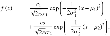 (7)where
 ,
,
 are the
variances, μ1, μ2 the mathematical
expectations and c1, c2 the
weights, and where we suppose
σ1 < σ2.
In addition, the most usual situation in catalog problems is
μ1 = μ2 = 0, and so, we make
this assumption (Even when we consider a more general case, the method is still valid as
we show in the Appendix). If we define
are the
variances, μ1, μ2 the mathematical
expectations and c1, c2 the
weights, and where we suppose
σ1 < σ2.
In addition, the most usual situation in catalog problems is
μ1 = μ2 = 0, and so, we make
this assumption (Even when we consider a more general case, the method is still valid as
we show in the Appendix). If we define 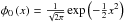 ,
then the kth-derivative is
,
then the kth-derivative is
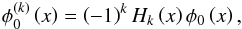 (8)where
Hk is the kth-Hermite’s
polynomial (Ayant 1971). (The sign is included for
convenience.) If we denote hk as the
corresponding kth-Hermite function, we obtain the following for the
derivatives of the Gaussian mixture:
(8)where
Hk is the kth-Hermite’s
polynomial (Ayant 1971). (The sign is included for
convenience.) If we denote hk as the
corresponding kth-Hermite function, we obtain the following for the
derivatives of the Gaussian mixture:
 (9)We consider the
properties of the Hermite functions:
(9)We consider the
properties of the Hermite functions:
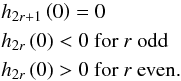 (10)For
k = 2r, we see that the summand containing the least
variance dominates:
(10)For
k = 2r, we see that the summand containing the least
variance dominates: ![\begin{equation} \begin{array}{c} \frac{f^{\left( k\right) }\left( x\right) }{\frac{c_{1}}{\sigma _{1}^{k+1}} h_{k}\left( \frac{x}{\sigma _{1}}\right) }=1+\frac{\frac{c_{2}}{c1}h\left( \frac{x}{\sigma 2}\right) }{\left( \frac{\sigma _{2}}{\sigma _{1}}\right) ^{k+1}h\left( \frac{x}{\sigma _{1}}\right) }\Rightarrow \\[2mm] \frac{f^{\left( k\right) }\left( 0\right) }{\frac{c_{1}}{\sigma _{1}^{k+1}} h_{k}\left( 0\right) }=1+\frac{\frac{c_{2}}{c1}}{\left( \frac{\sigma _{2}}{ \sigma _{1}}\right) ^{k+1}}\overset{k\rightarrow \infty }{\longrightarrow }1. \end{array} \end{equation}](/articles/aa/full_html/2013/10/aa21995-13/aa21995-13-eq51.png) (11)Since
we assumed μ1 = μ2 = 0 and
σ1 < σ2,
then it follows that f(2r) has a local
extreme (also absolute) at x = 0. To compute the estimation of the least
variance, it suffices to apply
(11)Since
we assumed μ1 = μ2 = 0 and
σ1 < σ2,
then it follows that f(2r) has a local
extreme (also absolute) at x = 0. To compute the estimation of the least
variance, it suffices to apply 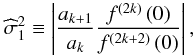 (12)where
ak is the independent term of
H2k. The computation of
(12)where
ak is the independent term of
H2k. The computation of
 follows from
 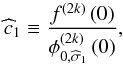 (13)where
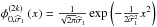 .
If we apply the previous formulas to the new function,
.
If we apply the previous formulas to the new function,
![\begin{equation} f^{[1] }\left( x\right) =f\left( x\right) -\frac{1}{\sqrt{2\pi } \widehat{\sigma }_{1}}\exp \left( -\frac{1}{2\widehat{\sigma }_{1}^{2}} x^{2}\right), \end{equation}](/articles/aa/full_html/2013/10/aa21995-13/aa21995-13-eq61.png) (14)then we obtain
(14)then we obtain
 Though the method used to deduce the different summands of a two-Gaussian mixture is
intuitive, we have introduced a brief formal proof of the most general case (considering
any μ1 and μ2, being them null or
not) in the Appendix.
Though the method used to deduce the different summands of a two-Gaussian mixture is
intuitive, we have introduced a brief formal proof of the most general case (considering
any μ1 and μ2, being them null or
not) in the Appendix.
3. Parameter estimation with intermediate nonparametric regression
In this section, we first consider a decomposition of the error estimation in two terms: a first term involving the mean squared of the bias and a second term with the variance. For a more complete exposition of this subject, see Cucker & Smale (2002).
The second subsection deals with nonparametric estimation of the coefficients belonging to an developing approach. One can conclude that different coefficients could be computed with different bandwidths. We can also observe that it is possible to compute different integrals, while evaluating them over a small set of points (for example in a Gaussian quadrature). Thus, the reconstruction of the required function (its finite development adding the total energy of the function) may be carried out using different bandwidths to compute nonparametric approximations in a reduced set of points, where integral evaluations are required. If a predetermined minimum total energy is not reached, the coefficient is rejected, and the next coefficient is tested. Obviously, higher harmonics could not be computed depending on the properties of the initial data set. These properties of the method may be used to take advantage if a development in a certain functional basis is required. It is also useful for the case of a geometrical expression of the signal, as we see in Sect. 5.
3.1. Decomposition of the error of the signal function
Let X,Y be random variables that we suppose are defined in a real
compact interval such as I1 and
I2, respectively. We suppose that we are searching for a model
y = f(x). The least squares error of
the model is given as
ε(f) = ερ(f) = ∫Z(y − f(x))2dρ,
where Z = I1 × I2
and dρ is a measure of probability for the bidimensional
RV(X, Y) . We suppose that we work with functions
ϕ(x, y) to whom Fubbini’s Theorem is applicable. Thus,
we name
dρX, dρ(y|x)
the marginal measure for X and the conditional of Y with
respect to X. We can apply
![\begin{equation} \int_{I_{1}\times I2}\varphi (x,y){\rm d}\rho =\int_{I_{1}}\left[ \int_{I_{2}}\varphi (x,y){\rm d}\rho _{Y\mid X\,=\,x}\right] {\rm d}\rho _{X}. \end{equation}](/articles/aa/full_html/2013/10/aa21995-13/aa21995-13-eq74.png) (15)We return to RV and
denote
(15)We return to RV and
denote ![\begin{equation} m_{\rho }(x)=\int_{I_{2}}y{\rm d}\rho _{Y \mid X\,=\,x}=E[Y\!\mid\! X\,=\,x]. \end{equation}](/articles/aa/full_html/2013/10/aa21995-13/aa21995-13-eq75.png) (16)Obviously, the
residual
y − mρ(x)
has a null mathematical expectation, and its variance is given by
(16)Obviously, the
residual
y − mρ(x)
has a null mathematical expectation, and its variance is given by
 (17)We denote the integral of
this variance as
(17)We denote the integral of
this variance as  . That is, it represents
the least square error of the regression function (with respect to the density
ρ). It is clear that we obtain the decomposition of the error that is
associated with an approximation
. That is, it represents
the least square error of the regression function (with respect to the density
ρ). It is clear that we obtain the decomposition of the error that is
associated with an approximation  of f, which provides the following after some algebraic operations:
 (18)In this identity
(18), we see that the first term depends on the regression function
mρ and the approximation
.
The last term is independent of the unknown; it depends only on the measure
ρ and is the lower bound of the error, since it does not depend on the
approximation as it is stated. In general, one can suppose that
mρ belongs to some functional space that
admits a development in the appropriate convergent series. On the other hand, different
approaches to the estimated function
are possible. The main question that appears concerns the bias. One can make many
assumptions about mρ and try different
methods to find .
We get mρ approaching the different densities
by means of a nonparametrical method. Nevertheless, other choices are possible. This
selection requires a consideration regarding bias and variance in the approximation
process (see following subsection). For the function
,
we select a complete Hilbert space (in such a way that it has a functional basis) or
Banach space with a basis or dictionary (not necessarily free with a possible redundant
generator system. An infinite series may be expressed in more than one way. This is not
our case, because we work with a finite sum of terms) to consider a nonlinear, m-term
approximation (sum of the m terms of the basis or the dictionary, depending on the
situation). The method to obtain the coefficients is considered below, and we get a rule
to diminish statistical bias.
(18)In this identity
(18), we see that the first term depends on the regression function
mρ and the approximation
.
The last term is independent of the unknown; it depends only on the measure
ρ and is the lower bound of the error, since it does not depend on the
approximation as it is stated. In general, one can suppose that
mρ belongs to some functional space that
admits a development in the appropriate convergent series. On the other hand, different
approaches to the estimated function
are possible. The main question that appears concerns the bias. One can make many
assumptions about mρ and try different
methods to find .
We get mρ approaching the different densities
by means of a nonparametrical method. Nevertheless, other choices are possible. This
selection requires a consideration regarding bias and variance in the approximation
process (see following subsection). For the function
,
we select a complete Hilbert space (in such a way that it has a functional basis) or
Banach space with a basis or dictionary (not necessarily free with a possible redundant
generator system. An infinite series may be expressed in more than one way. This is not
our case, because we work with a finite sum of terms) to consider a nonlinear, m-term
approximation (sum of the m terms of the basis or the dictionary, depending on the
situation). The method to obtain the coefficients is considered below, and we get a rule
to diminish statistical bias.
The classical approach to the regression problem may be considered a particular case of
the previous one. After selecting the working functional space H, we
consider  , where
(xi,yi),
1 ≤ i ≤ n represents the finite sample. The
decomposition formulas are theoretically similar, but the implementation is different, and
there are very important differences between both methods. We prefer the former approach
and we explain its advantages in the following section. In addition, we can mention other
advantages, such as a) a more robust approach; b) the lack of need to choose an a priori
model and c) an approximation of the density function (which generalizes the assignment of
weights). It is interesting to remark that the classical method may provide wrong results,
if the abscises are, for instance, inhomogeneously distributed. Another problem consists
of requiring the recomputation of the coefficients in a model of adjustment when its order
is increased, because the coefficients of lower orders are not preserved. The main problem
of nonparametrical methods is related with the bandwidth selected value. Nevertheless,
there are very accurate methods to solve this problem, considering the complete
statistical information of the data. Another problem is the missed geometrical-analytical
sense. The earlier problem is overcome when we take the nonparametrical method as an
intermediate adjustment, because it contains complete statistical information of the data
by means of estimating the density function.
, where
(xi,yi),
1 ≤ i ≤ n represents the finite sample. The
decomposition formulas are theoretically similar, but the implementation is different, and
there are very important differences between both methods. We prefer the former approach
and we explain its advantages in the following section. In addition, we can mention other
advantages, such as a) a more robust approach; b) the lack of need to choose an a priori
model and c) an approximation of the density function (which generalizes the assignment of
weights). It is interesting to remark that the classical method may provide wrong results,
if the abscises are, for instance, inhomogeneously distributed. Another problem consists
of requiring the recomputation of the coefficients in a model of adjustment when its order
is increased, because the coefficients of lower orders are not preserved. The main problem
of nonparametrical methods is related with the bandwidth selected value. Nevertheless,
there are very accurate methods to solve this problem, considering the complete
statistical information of the data. Another problem is the missed geometrical-analytical
sense. The earlier problem is overcome when we take the nonparametrical method as an
intermediate adjustment, because it contains complete statistical information of the data
by means of estimating the density function.
3.2. Mixed methods
The range of the covariant values (the sample of the RV X in this Sect.
3) could be an inhomogeneous distribution. If we nevertheless take a nonparametric
adjustment, it is possible to use it to compute the estimation of the function in an
arbitrary point. This implies that we could extend the function values regularly over the
complete domain. To highlight its advantage, we consider a simple example: if we suppose,
for example, that the function f belongs to a separable Hilbert space
with a complete orthonormal basis
{φi > 0, i ≥ 0},
then we have a unique expansion  (19)The computation of
each coefficient could be performed using
(19)The computation of
each coefficient could be performed using  with ⟨|⟩ being the inner product in the space and
  the nonparametric (intermediate) estimation. The inner product could be approximated by a
numerical integration method to be as accurate as necessary. If we consider, for example,
a Gauss-type method, we must estimate the value of the function in a few number of points.
Furthermore, there are different methods, which are specially prepared to estimate the
optimal bandwidth for each point, which must be taken. For more information about
nonparametrical methods, see Wand & Jones (1995). As previously mentioned, it is equally possible to estimate the
coefficients of a geometrical model of adjustment, as we see in Sect. 5.
the nonparametric (intermediate) estimation. The inner product could be approximated by a
numerical integration method to be as accurate as necessary. If we consider, for example,
a Gauss-type method, we must estimate the value of the function in a few number of points.
Furthermore, there are different methods, which are specially prepared to estimate the
optimal bandwidth for each point, which must be taken. For more information about
nonparametrical methods, see Wand & Jones (1995). As previously mentioned, it is equally possible to estimate the
coefficients of a geometrical model of adjustment, as we see in Sect. 5.
There is another advantage when a coefficient of a harmonic must be computed. Not only is this due to the former property but also this procedure does not make any supposition regarding the order of the actual expansion. In this sense, our method is not linear and it is possible to expand it to a great number of problems.
3.3. Nonparametrical estimation of coefficients of minimum energy in the Fourier case
We suppose developments
m(x) = ∑ ckϕk(x)
and  . Along this subsection we
neglect, unlike the previous section, the dependence of the density ρ.
The mathematical expectation of the coefficients is given by
. Along this subsection we
neglect, unlike the previous section, the dependence of the density ρ.
The mathematical expectation of the coefficients is given by
![\begin{equation} E[\widehat{c}_{k}|X_{1},....,X_{n}]=\int_{ \mathbb{R} ^{n}}\widehat{c}_{k}f(x_{1},...,x_{n}){\rm d}x_{1},...{\rm d}x_{n}, \end{equation}](/articles/aa/full_html/2013/10/aa21995-13/aa21995-13-eq95.png) (20)where
X1,....,Xn
is a set of independent random variables distributed identically like X,
and f is its joint density function. We apply the relation between the
coefficients, the basis, and the function:
(20)where
X1,....,Xn
is a set of independent random variables distributed identically like X,
and f is its joint density function. We apply the relation between the
coefficients, the basis, and the function:
 (21)where
we have applied Fubbini’s theorem. By definition, we have this transformation:
(21)where
we have applied Fubbini’s theorem. By definition, we have this transformation:
![\begin{eqnarray} &&\int_{ \mathbb{R} }E[\widehat{m}(x)|X_{1},...,X_{n}]\varphi _{k}(x){\rm d}x= \notag \\ &&c_{k}+\int_{ \mathbb{R} }E[\widehat{m}(x)-m(x)|X_{1},...,X_{n}]\varphi _{k}(x){\rm d}x. \end{eqnarray}](/articles/aa/full_html/2013/10/aa21995-13/aa21995-13-eq99.png) (22)If
we take a local polynomial kernel regression of third order and a Fourier series is
considered, then we have
(22)If
we take a local polynomial kernel regression of third order and a Fourier series is
considered, then we have ![\begin{equation} E[\widehat{c}_{k}|X_{1},....,X_{n}]=c_{k}\left(1+\alpha \frac{(kh)^{4}}{24}\right), \end{equation}](/articles/aa/full_html/2013/10/aa21995-13/aa21995-13-eq100.png) (23)where α
is a constant depending only on the used kernel, h is the bandwidth, see
Fan & Gijbels (1992), and k
is the order of the considered harmonic. This expression makes it clear: if
h1 is a good selection for the
c1 term, then
(23)where α
is a constant depending only on the used kernel, h is the bandwidth, see
Fan & Gijbels (1992), and k
is the order of the considered harmonic. This expression makes it clear: if
h1 is a good selection for the
c1 term, then  can be used
to approach the ck coefficient with the same
reliability,
can be used
to approach the ck coefficient with the same
reliability,  . For
numerical purposes, this property may be of interest.
. For
numerical purposes, this property may be of interest.
4. Parametrical regression methods
The different adjustment methods have been widely described in other papers and we do not repeat them here. We only mention
that different parametrical methods provide different adjustment models, following different hypotheses: These methods present some advantages and some problems. The main advantage is that they provide a (primary) qualitative explanation for the errors, and it is also possible to include other parameters with physical meaning.
In contrast, there are some initial problems: in many cases, the selected model is not representative of the problem and even more importantly, an inhomogeneous spatial distribution of the set of data implies instability to compute the parameters directly. Even using high orders, the results are not realistic if we have few stars. If higher order harmonics appear in the spherical harmonics case, the usual method could be wrong.
5. Using two different quasar catalogs to improve the ICRF-Ext2
As a numerical application of the previous sections, we have considered two input catalogs: the USNO and JPL, which contain 189 common defining sources from the ICRF-Ext2 catalog. They were submitted by JPL (Caltech/NASA Jet Propulsion Laboratory, USA), and USNO (US Naval Observatory, USA). A brief description of the input catalogs is given in Table 1 (Sokolova & Malkin 2007).
This section is divided into two subsections. The first one concerns the process of building a combined catalog from the two chosen input catalogs. In the second subsection, we propose a procedure of acceptation from candidate sources to reference sources. We check that the candidate sources selected using our method from the ICRS-Ext2 are indeed included in the ICRF2 as defining or non defining sources.
Input catalogs.
5.1. The use of JPL and USNO catalogs to build a combined catalog
In this study, we considered only the sources which have at least 15 observations in two sessions. We have not included some reference sources in our calculus that present oddly high residuals. All values are given in μas. The values of the initial arithmetic mean μ and standard deviation σ are as follows: for the USNO catalog, they are μα = 10.2 and σα = 246.8, μδ = −5.2 and σδ = 307.5. For the JPL catalog they are μα = −32.6 and σα = 341.5, μδ = −12.1 and σδ = 354.4. It seems that JPL is not completely homogeneous as defined in Sect. 2 and it could require a more careful study. We have included it in our adjustment, because it serves to show the strength of our method.
With respect to the study of the residuals, we have chosen to carry out a preliminary
kernel nonparametric (KNP henceforth) adjustment for the
Δα cosδ and Δδ in both catalogs and
a vectorial spherical harmonics (VSH henceforth) of first order for the adjustment model
(25). Then, we apply our mixed method as it has been explained in Sects. 3.1 and 3.2 by
taking ![\hbox{$ m_{\rho }=[\Delta \alpha \,\cos \delta ,\Delta \delta ] ^{t}, \widehat{m}=[m_{\alpha },m_{\delta }] ^{t}$}](/articles/aa/full_html/2013/10/aa21995-13/aa21995-13-eq126.png) for each catalog in
the first summand of the expression (18). The existence of deformations has required the
use of a correction for each catalog given by
for each catalog in
the first summand of the expression (18). The existence of deformations has required the
use of a correction for each catalog given by
![\begin{equation} \begin{array}{c} \underset{C^{i}}{\min }\int_{S^{2}}\left\{ [\left( \Delta \alpha \cos \delta \right) ^{\left( i\right) }-m_{\alpha }^{[i] }\left( \alpha ,\delta \right) ] ^{2}+\right. \\ \\ \left. [\left( \Delta \delta \right) ^{\left( i\right) }-m_{\delta }^{ [i] }\left( \alpha ,\delta \right) ] ^{2}\right\} {\rm d}S, \end{array} \end{equation}](/articles/aa/full_html/2013/10/aa21995-13/aa21995-13-eq127.png) (27)where
Ci are the coefficients of the models
(27)where
Ci are the coefficients of the models
![\hbox{$ m_{\alpha }^{[i]}$}](/articles/aa/full_html/2013/10/aa21995-13/aa21995-13-eq129.png) and
and
![\hbox{$m_{\delta }^{[i]}$}](/articles/aa/full_html/2013/10/aa21995-13/aa21995-13-eq130.png) with i = 1 (USNO) and i = 2 (JPL). The results for
the coefficients of the VSH of first order are listed in the Table 2, where it can be seen that JPL provides high coefficients for the
deformation. This must be considered in future studies. The coefficients listed in Table
2 are obtained by applying condition (27) and
solving the resulting normal equations. They consist of different integrals, which are
evaluated over a grid of equidistant points over the sphere where the KNP values for
Δα cosδ and Δδ are computed.
with i = 1 (USNO) and i = 2 (JPL). The results for
the coefficients of the VSH of first order are listed in the Table 2, where it can be seen that JPL provides high coefficients for the
deformation. This must be considered in future studies. The coefficients listed in Table
2 are obtained by applying condition (27) and
solving the resulting normal equations. They consist of different integrals, which are
evaluated over a grid of equidistant points over the sphere where the KNP values for
Δα cosδ and Δδ are computed.
Rotation and deformation parameters for the USNO and JPL in μas.
Next, we consider only the rotations. We subtract the corrections provided by the
rotations to the initial position to obtain the intermediate catalogs
USNO1 and
JPL1:
Cat1 = Cat − correction,
where these corrections depend only on the rotations. The adjustment itself is given by
![\begin{eqnarray} cat_{1}^{1}-(ICRF-Ext2) &=&m^{[1,1] }+\varepsilon ^{[1,1] } \notag \\ cat_{2}^{1}-(ICRF-Ext2) &=&m^{[2,1] }+\varepsilon ^{[2,1] }. \end{eqnarray}](/articles/aa/full_html/2013/10/aa21995-13/aa21995-13-eq143.png) (28)We
use now the term WRMS that denotes weighted root mean squared. In our case, the function
uses the weights assigned by the KNP adjustment. With regard to the WRMS in the entire
sphere where we have used numerical integration and a KNP adjustment, the initial WRMS in
right ascension is 61.1 and the final value is 36.4. The initial WRMS in declination is
113.9, and the final value is 47.9 for the USNO. The initial WRMS in right ascension is
99.5, and the final value is 61, while the initial WRMS in declination is 87.3, and the
final value is 78.7 for the JPL. A clear summary of these data may be seen in Table 3.
(28)We
use now the term WRMS that denotes weighted root mean squared. In our case, the function
uses the weights assigned by the KNP adjustment. With regard to the WRMS in the entire
sphere where we have used numerical integration and a KNP adjustment, the initial WRMS in
right ascension is 61.1 and the final value is 36.4. The initial WRMS in declination is
113.9, and the final value is 47.9 for the USNO. The initial WRMS in right ascension is
99.5, and the final value is 61, while the initial WRMS in declination is 87.3, and the
final value is 78.7 for the JPL. A clear summary of these data may be seen in Table 3.
Mean squared errors over the sphere after rotation adjustment.
 |
Fig. 1 Differences in (ICRF-Ext2)-USNO for Δα cosδ (in μas). The clear surface represents the initial differences, the dark surface represents the differences after the correction given by the rotations. Notice the rank for differences in Δα cosδ. |
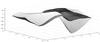 |
Fig. 2 Differences in (ICRF-Ext2)-USNO for the Δδ (in μas). The clear surface represents the initial differences, the dark surface represents the differences after the correction given by the rotations. |
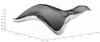 |
Fig. 3 Differences in (ICRF-Ext2)-JPL for the Δα cosδ (in μas). The clear surface represents the initial differences, the dark surface represents the differences after the correction given by the rotations. |
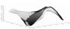 |
Fig. 4 Differences in (ICRF-Ext2)-JPL for the Δδ (in μas). The clear surface represents the initial differences; the dark surface represents the differences after the correction given by the rotations. |
The residual noise obtained after the adjustment (for each Δα cosδ, Δδ) may be observed in Figs. 1 to 4.
Prior to proceeding with the proposal of a combined catalog, we consider an example to show that our method detects inhomogenities (in the second sense given in Sect. 2) in building a combined catalog. Taking 0.5m[1,1] + 0.5m[2,1] only for Δα cosδ residuals belonging to the USNO and the JPL catalogs, the corresponding error is 0.5ε[1,1] + 0.5ε[2,1], which distributes as a Gaussian mixture with weights c1 = c2 = 0.5, standard deviations σ1 = 36.4, σ2 = 53.7, and mathematical expectations μ1 = 7.4, μ2 = −1.4. We use the procedures described in Sect. 2. As the use of high orders derivative has been necessary, we have introduced some variations. To ensure the results, we build a third order local KNP over equally spaced points and consider this function over more points to progressively increase the order of the local KNP (depending on the required precision to stabilize the desired decimal digit). Alternatively, we have applied formulas (12) and (13) for k = 0,2,4,6 and an Aitken approximation to obtain μ1 = 7.4, σ1 = 36.3, c1 = 0.5, μ2 = −1.4, σ2 = 53.7, and c2 = 0.5. This means that we have obtained the two populations used in the compilation of the combined catalog. We conclude that the construction of the compiled catalog has not been homogeneous in the second definition as given in Sect. 2.
Returning to the aim of compiling a combined catalog, we take the weights proposed by (4). The final residuals may be seen in Figs. 5 and 6. The final WRMS for the residuals are 35.6 for the right ascension and 41 for the declination.
5.2. Method to densify the reference
Finally, we propose a procedure to densify the reference frame. We work with the candidate sources of the ICRF-Ext2, but it could be also applied to other sources. For this purpose, we apply a simple test to discover if a source belongs to a determined population. The procedure is as follows: the obtained combined catalog provides residuals for Δα cosδ and Δδ distributed as N(0, 35.6) and N(0, 41.0) respectively. The corresponding density functions are Gaussians, and we can consider, for example, a 30% of the area centered on the corresponding mean (the radius of each interval is determined by each standard deviation). This area is bounded by the function and two abscises that represent errors in μas. If the expected error for a candidate source is comprised in the mentioned interval, it is reasonable for this candidate to be considered as a new reference source. In any case, a more strict condition is considered in the next steps.
Considering the previous guidelines, each final function of residuals for Δαcosδ and Δδ is a surface. Thus, we can project its contour lines in the XY plane. In particular, we focus on the contour lines signaled by the extremes of the intervals mentioned in the previous paragraph. This may also be applied individually for each catalog, and each individual candidate source of the catalogs. The steps to follow are
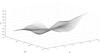 |
Fig. 5 Residuals in the final combined catalog for the Δα cosδ (in μas). |
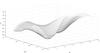 |
Fig. 6 Residuals in the final combined catalog for the Δδ (in μas). |
Selected candidate sources.
The verification using new catalogs may lead to the definitive choice of the source. In our case, we obtain the candidate sources listed in Table 4, where the names and the proposed position are given. It is remarkable that sources 1, 2 and 3 have been included among the 922 ICRF2 non-defining sources, while sources 4 and 5 have been included among the 295 defining sources of the ICRF2 (Fey et al. 2009).
6. Conclusions
The compilation of a large quasar catalog from other input catalogs is an important trend in the astronomical context. In this sense, it is interesting to study the initial catalogs, compared to the main catalog (in our case, the ICRF-Ext2 Catalog), to determine its inner homogeneity. To obtain a homogeneous combined catalog, it is necessary to use adequate weights. Reciprocally, it is possible to determine if a combined catalog has been obtained homogeneously or not. To this aim, we have studied both subjects in Sect. 2, which have been applied in Sect. 5.
A mixed method using nonparametrical regression to build an intermediate catalog presents many advantages to obtain accurate parameters. These advantages are as follows: a) a more robust approach in the sense that the computation of the coefficients is carried out by means of functional scalar products over the sphere. The homogeneous grid selection preserves the functional orthogonality in the process of discretization. b) There is no need to choose an a priori model. c) The approximation of the density function by means of a KNP (which generalizes the assignment of weights). These subjects have been studied in Sect. 3, and we can remark that different parametrical methods (geometric or analytic) may be employed to study global and local properties of the used catalogs to obtain a very good compiled catalog. In Sect. 4, we have briefly described the most currently parametrical models of adjustment.
The mixed method with an adequate weights selection has provided us a combined catalog with little final residuals, as seen in text.
We have also proposed a method to decide if a given candidate source may be coherently accepted as a new reference source with the obtained results for the combined catalog. The five sources proposed using our method have been included in the ICRF2, which includes two new defining sources and supports the reliability of our methods. Further studies may be carried out to explore other cases. For example, one can conduct a deeper study using surface or vectorial spherical harmonics of high orders. We can also include other input catalogs in the computation, which would not affect the method.
Acknowledgments
Part of this work was supported by a grant P1-1B2009-07 from Fundacio Caixa Castello BANCAIXA and a grant P1-061I455.01/1 from Bancaja.
References
- Arias, E. F., Feissel, M., & Lestrade, J. F. 1988, Annual Report for 1987, Observatoire de Paris, Paris, D-113 [Google Scholar]
- Arias, E. F., Charlot, P., Feissel, M., Lestrade, & Lestrade, J. F. 1995, A&A, 303, 604 [NASA ADS] [Google Scholar]
- Ayant, Y., & Borg, M. 1971, Fonctions spéciales à l’usage des étudiants en physique (Paris: Dunod) [Google Scholar]
- Cucker, F., & Smale, S. 2002, Bull. A.M.S., 39, 1 [Google Scholar]
- Fan, J., & Gijbels, I. 1992, Ann. Statist. 20, 4, 2008 [CrossRef] [Google Scholar]
- Feissel, M., & Mignard, F. 1998, A&A, 331, L33 [Google Scholar]
- Fey, A. L., Ma, C., Arias, E. F., et al. 2004, AJ, 127, 3587 [NASA ADS] [CrossRef] [Google Scholar]
- Fey, A., Gordon, D., & Jacobs, C. 2009, IERS Technical Note 35, The Second realization of the International Celestial Reference Frame by Very Long Baseline Interferometry, Frankfurt am Main 2010: Verlag des Bundesamts für Kartographie und Geodäsie [Google Scholar]
- IERS 1999, 1998 IERS Annual Report, Observatoire de Paris, D. Gambis (Editor) [Google Scholar]
- Heiskanen, W. A., & Moritz H. 1967, Physical Geodesy (San Francisco: Freeman) [Google Scholar]
- Ma, C., Arias, E. F., Eubanks, T. M., et al. 1998, AJ, 116, 516 [NASA ADS] [CrossRef] [Google Scholar]
- Marco, F., Marco, F. J., Martínez, M. J., & López, J. A. 2004a, A&A, 418, 1159 [NASA ADS] [CrossRef] [EDP Sciences] [Google Scholar]
- Marco, F., Marco, F. J., Martínez, M. J., & López, J. A. 2004b, AJ, 127, 549 [NASA ADS] [CrossRef] [Google Scholar]
- Martínez, M. J., Marco, F. J., & López, J. A. 2009, Pub. ASP, 121, 167 [NASA ADS] [Google Scholar]
- Sfikas et al. 2005, in ICANN 2005, LNCS 3697, eds. W. Duch et al., 835 [Google Scholar]
- Sokolova, Ju., & Malkin, Z. 2007, A&A, 474, 2, 665 [NASA ADS] [CrossRef] [EDP Sciences] [Google Scholar]
- Walter, H. G. 1989a, A&A, 210, 455 [NASA ADS] [Google Scholar]
- Walter, H. G. 1989b, A&A, 79, 283 [Google Scholar]
- Walter, S., & Sovers, O. J. 2000, Astrometry of fundamental catalogs. The evolution from optical to radio reference frames (Berlin: Springer-Verlag) [Google Scholar]
- Wand, M. P., & Jones, M. C. 1995, Kernel Smoothing (London: Chapman and Hall) [Google Scholar]
- Yatskiv, YA S., & Kuryakova. 1990, in Inertial Coordinate System on the Sky, Proc. 141th, eds. J.H. Lieske, & V. K. Abalakin, IAU Symp., 295 [Google Scholar]
- Yu, M., Manchester, R. N., Hobbs, G., et al. 2013, MNRAS, 429, 688 [NASA ADS] [CrossRef] [Google Scholar]
Appendix A:
Lemma 1: let f,g be continuous and derivable in a given interval with
the possible exception of a finite number of points. Let us assume that
f(a) = g(a) and
f′(a) = g′(a),
which verifies:  If
we suppose that
α(x) > β(x),
then Proof of a):
If
we suppose that
α(x) > β(x),
then Proof of a):
If we multiply the first equation by g(x), the second
by f(x), and then we subtract, we get
 (A.3)Given any
x where
a < x ≤ c, we
integrate both members of the equality:
(A.3)Given any
x where
a < x ≤ c, we
integrate both members of the equality:
![\appendix \setcounter{section}{1} \begin{eqnarray} &&\int_{a}^{x}[f^{\prime \prime }(x)g(x)-g^{\prime \prime }(x)f(x)] {\rm d}x=\notag \\ &&\int_{a}^{x}(\beta (x)-\alpha (x))f(x)g(x){\rm d}x<0 \end{eqnarray}](/articles/aa/full_html/2013/10/aa21995-13/aa21995-13-eq205.png) (A.4)and
we obtain:
(A.4)and
we obtain: 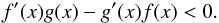 (A.5)Thus,
 is a strict decreasing function that reaches a value one for
x = a. It is then necessary that
f(x) < g(x)
for x > a , because both
functions are positive in the subinterval.
is a strict decreasing function that reaches a value one for
x = a. It is then necessary that
f(x) < g(x)
for x > a , because both
functions are positive in the subinterval.
Proof of b) We follow the development of Lemma 1 until we arrive at
 (A.6)since we assume that
g(x) < 0, then
g(x) < f(x).
(A.6)since we assume that
g(x) < 0, then
g(x) < f(x).
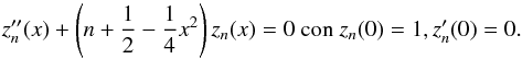
Note: let us suppose the differential equation  , where
 . Then
 in the
interval of definition. It is evident that this result is equally true for function
f.
in the
interval of definition. It is evident that this result is equally true for function
f.
Proof of c) For the subinterval [a,c] we can apply a). For the
subinterval [c,d], we consider function
 from
the former note. Following the steps of the proof given in a), we have for each
x, where
c < x < d:
from
the former note. Following the steps of the proof given in a), we have for each
x, where
c < x < d:
![\appendix \setcounter{section}{1} \begin{eqnarray} &&\int_{x}^{d}[f^{\prime \prime }(x)\widetilde{g}(x)-\widetilde{g} ^{\prime \prime }(x)f(x)] {\rm d}x = \notag \\ &&\int_{x}^{d}(\beta (x)-\alpha (x))f(x)\widetilde{g}(x){\rm d}x < 0. \end{eqnarray}](/articles/aa/full_html/2013/10/aa21995-13/aa21995-13-eq218.png) (A.7)In
(c,d), we have
(A.7)In
(c,d), we have  . Therefore,
![\appendix \setcounter{section}{1} \begin{equation} [f^{\prime }(d)\widetilde{g}(d)-\widetilde{g}^{\prime }(d)f(d)] - [f^{\prime }(x)\widetilde{g}(x)-\widetilde{g}^{\prime }(x)f(x)] <0. \end{equation}](/articles/aa/full_html/2013/10/aa21995-13/aa21995-13-eq221.png) (A.8)Hence,
(A.8)Hence,
![\appendix \setcounter{section}{1} \begin{equation} [f^{\prime }(x)\widetilde{g}(x)-\widetilde{g}^{\prime }(x)f(x)] >-\widetilde{g}^{\prime }(d)f(d)>0, \end{equation}](/articles/aa/full_html/2013/10/aa21995-13/aa21995-13-eq222.png) (A.9)because
f(d) < 0 and
(A.9)because
f(d) < 0 and
 . With this, we deduct that
 is decreasing in (c,d) with the quotient null in
x = c and both expressions are negative, reaching the
maximum at x = d. Thus,
is decreasing in (c,d) with the quotient null in
x = c and both expressions are negative, reaching the
maximum at x = d. Thus,
 for
c < x < d.
In addition, if
for
c < x < d.
In addition, if  , then
 , and we
would obtain
, and we
would obtain  , which
is absurd. Consequently,
, which
is absurd. Consequently,  (A.10)Thus, function
f(x) verifies
− g(x) ≤ f(x) ≤ g(x)
between two consecutive extremes of f. This argument may be extended to
all real domain.
(A.10)Thus, function
f(x) verifies
− g(x) ≤ f(x) ≤ g(x)
between two consecutive extremes of f. This argument may be extended to
all real domain.
Corollary 1: we assume the same general conditions about f and g from the former Lemma. If the first differential equations have been verified with β > 0, g > 0, and β ≤ α and we have the additional conditions f(a) = g(a), f′(a) = g′(a) or f(a) = −g(a), f′(a) = −g′(a) then |f(x)| ≤ g(x) for x ∈ [a,b] .
Lemma 2: let  where
n = 2r (which includes the particular case
n = 4r). Then, it is verified that
where
n = 2r (which includes the particular case
n = 4r). Then, it is verified that
Proposition 1: let  with α > 0. Then we have for any
x that
with α > 0. Then we have for any
x that  for a
certain α > 0. For example,
for a
certain α > 0. For example,
 .
The value of α may be provided with more accuracy: α is
a value such that the inflection point of
h2(x), as indicated in
.
The value of α may be provided with more accuracy: α is
a value such that the inflection point of
h2(x), as indicated in
 ,
is a common point for both functions, which provides α ≈ 4.4234, a very
close value to
,
is a common point for both functions, which provides α ≈ 4.4234, a very
close value to  Proof: considering that function g verifies that
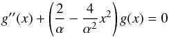 (A.11)and
g(0) = 1,g′(0) = 0, we
apply corollary 1 if
(A.11)and
g(0) = 1,g′(0) = 0, we
apply corollary 1 if  (A.12)The least value of the
second member of the inequality is obtained for n = 2, (when
x is fixed), and we obtain the sufficient condition:
(A.12)The least value of the
second member of the inequality is obtained for n = 2, (when
x is fixed), and we obtain the sufficient condition:
 (A.13)This may be immediately
verified: if we take, for example,
(A.13)This may be immediately
verified: if we take, for example,  ,
the inequality verifies for x ≤ 41. For higher values of
x, g(x) and
zn(x) are negligible for
any desired accuracy.
,
the inequality verifies for x ≤ 41. For higher values of
x, g(x) and
zn(x) are negligible for
any desired accuracy.
Proposition 2: let h2r,1 the first positive
zero of the Hermite function
h2r(x). We have that
(Ayant 1971)
 (A.14)
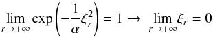
Theorem 1: let 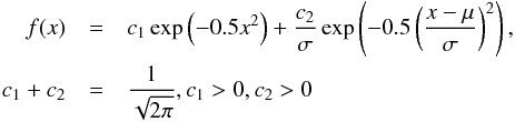 (A.15)and
let us suppose that σ > 1. Then if we denote
ξr as the point on the
x-axis where the higher relative extreme is in absolute value of the
2r-th derivative of f, we have that
(A.15)and
let us suppose that σ > 1. Then if we denote
ξr as the point on the
x-axis where the higher relative extreme is in absolute value of the
2r-th derivative of f, we have that
 (A.16)
Proof: to enable the proofs, we take 4r, instead of 2r,
because we can work with positive maximum without loss of generality in this case. Let us
suppose that
f(4r)(ξr) > 0
and also that ξr > 0.
First, note that  (A.17)and,
dividing by
c1h4r(0), we have
(A.17)and,
dividing by
c1h4r(0), we have
 (A.18)With this, we have the
following boundary for any x:
(A.18)With this, we have the
following boundary for any x:
 (A.19)because
σ > 1 and
h4r(x) reaches the
absolute maximum at x = 0. This indicates that the first summand in the
decomposition of f(4r)(x) is
dominant. We see that this idea is confirmed in the announced asymptotic result. Given the
former considerations, it is immediate that, there is a r1 for
any given ε1 > 0 such that
(A.19)because
σ > 1 and
h4r(x) reaches the
absolute maximum at x = 0. This indicates that the first summand in the
decomposition of f(4r)(x) is
dominant. We see that this idea is confirmed in the announced asymptotic result. Given the
former considerations, it is immediate that, there is a r1 for
any given ε1 > 0 such that
 (A.20)for
r ≥ r1 with an independence of
x. In particular, we have
(A.20)for
r ≥ r1 with an independence of
x. In particular, we have
 (A.21)We have
f(4r)(ξr) > 0,
and the previous bound assures that the quotient
(A.21)We have
f(4r)(ξr) > 0,
and the previous bound assures that the quotient  is positive. Considering the first proposition, we know that
 for a
certain α > 0, so
for a
certain α > 0, so
 (A.22)Now, let us
suppose that
(A.22)Now, let us
suppose that  with
h4r,1 being the first positive zero of
h4r(x). Then
with
h4r,1 being the first positive zero of
h4r(x). Then
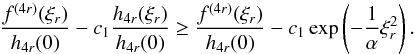
 (A.23)From
(A.22) and (A.23),
(A.23)From
(A.22) and (A.23), 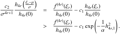 (A.24)Because
we suppose that ξr is the absolute positive
maximum of f(4r)(x), we can
deduct that there is a ε(r) value such that:
(A.24)Because
we suppose that ξr is the absolute positive
maximum of f(4r)(x), we can
deduct that there is a ε(r) value such that:
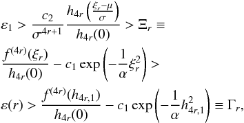 (A.25)where
we have applied (A.24). The ε(r) value separates the
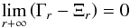
different values of Ξr and Γr. Two
contrasting situations may appear: either
(A.25)where
we have applied (A.24). The ε(r) value separates the
different values of Ξr and Γr. Two
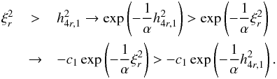
contrasting situations may appear: either or
or
 , which corresponds,
as we see, with the case
0 < ξr < h4r, 1 for
r > r1. Let us
check that we already have the desired result. The first case is incompatible with the
free choice of ε1, which could be taken as
ε1 < ε0.
Thus, it should accomplish that
, which corresponds,
as we see, with the case
0 < ξr < h4r, 1 for
r > r1. Let us
check that we already have the desired result. The first case is incompatible with the
free choice of ε1, which could be taken as
ε1 < ε0.
Thus, it should accomplish that  (A.26)and then
 (A.27)with the limits being
finite in both expressions. Consequently, we consider Proposition 2 and we have:
(A.27)with the limits being
finite in both expressions. Consequently, we consider Proposition 2 and we have:
![\appendix \setcounter{section}{1} \begin{eqnarray} \underset{r\rightarrow +\infty }{\lim }\Gamma _{r} &=& \underset{r\rightarrow +\infty }{\lim }\left[ \frac{f^{(4r)}(h_{4r,1})}{h_{4r}(0)}-c_{1}\exp \left(- \frac{1}{\alpha }h_{4r,1}^{2}\right)\right] \notag \\ &=&\underset{r\rightarrow +\infty } {\lim}\left[ \frac{f^{(4r)}(0)}{h_{4r}(0)} -c_{1}\right] , \end{eqnarray}](/articles/aa/full_html/2013/10/aa21995-13/aa21995-13-eq305.png) (A.28)which
implies that
(A.28)which
implies that  is finite, and
 ![\appendix \setcounter{section}{1} \begin{eqnarray} \left[ \underset{r\rightarrow +\infty }{\lim }\frac{f^{(4r)}(0)}{h_{4r}(0)} \right] -c_{1} &=&\underset{r+\infty }{\lim }\Xi _{r} \\ &=&\underset{r\rightarrow +\infty }{\lim }\left[ \frac{f^{(4r)}(\xi _{r})}{ h_{4r}(0)}-c_{1}\exp \left(-\frac{1}{\alpha }\xi _{r}^{2}\right)\right]. \nonumber \end{eqnarray}](/articles/aa/full_html/2013/10/aa21995-13/aa21995-13-eq307.png) (A.29)The
existence of finite limits allow us to rewrite them as
(A.29)The
existence of finite limits allow us to rewrite them as
![\appendix \setcounter{section}{1} \begin{eqnarray} 0 &\leq &\underset{r\rightarrow +\infty }{\lim }\frac{f^{(4r)}(\xi _{r})-f^{(4r)}(0)}{h_{4r}(0)} \\ &=&\underset{r\rightarrow +\infty }{\lim }c_{1}\left[ \exp \left(-\frac{1}{\alpha }\xi _{r}^{2}\right)-1\right] \leq 0. \nonumber \end{eqnarray}](/articles/aa/full_html/2013/10/aa21995-13/aa21995-13-eq308.png) (A.30)The
limit on the left is equal or greater to zero because it is finite, the denominator is
positive, and ξr is the point where
f(4r)(x) is maximum (and
positive). The second member of the equality is equal to or less than zero, because
(A.30)The
limit on the left is equal or greater to zero because it is finite, the denominator is
positive, and ξr is the point where
f(4r)(x) is maximum (and
positive). The second member of the equality is equal to or less than zero, because
 y
c1 ≥ 0. In conclusion, only one possibility remains:
y
c1 ≥ 0. In conclusion, only one possibility remains:
 (A.31)which we wanted to prove.
Theorem 2: let 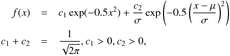 (A.32)and
let us suppose that σ < 1. If we denote
ξr as the point on the
x-axis where the higher relative extreme is in absolute value of the
2r-th derivative of f, we have that:
(A.32)and
let us suppose that σ < 1. If we denote
ξr as the point on the
x-axis where the higher relative extreme is in absolute value of the
2r-th derivative of f, we have that:
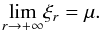 (A.33)
All Tables
All Figures
|
Fig. 1 Differences in (ICRF-Ext2)-USNO for Δα cosδ (in μas). The clear surface represents the initial differences, the dark surface represents the differences after the correction given by the rotations. Notice the rank for differences in Δα cosδ. |
| In the text | |
|
Fig. 2 Differences in (ICRF-Ext2)-USNO for the Δδ (in μas). The clear surface represents the initial differences, the dark surface represents the differences after the correction given by the rotations. |
| In the text | |
|
Fig. 3 Differences in (ICRF-Ext2)-JPL for the Δα cosδ (in μas). The clear surface represents the initial differences, the dark surface represents the differences after the correction given by the rotations. |
| In the text | |
|
Fig. 4 Differences in (ICRF-Ext2)-JPL for the Δδ (in μas). The clear surface represents the initial differences; the dark surface represents the differences after the correction given by the rotations. |
| In the text | |
|
Fig. 5 Residuals in the final combined catalog for the Δα cosδ (in μas). |
| In the text | |
|
Fig. 6 Residuals in the final combined catalog for the Δδ (in μas). |
| In the text | |
Current usage metrics show cumulative count of Article Views (full-text article views including HTML views, PDF and ePub downloads, according to the available data) and Abstracts Views on Vision4Press platform.
Data correspond to usage on the plateform after 2015. The current usage metrics is available 48-96 hours after online publication and is updated daily on week days.
Initial download of the metrics may take a while.