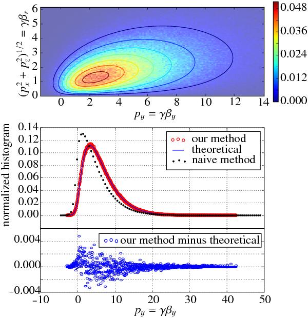
Fig. 9
Maxwell-Jüttner distribution for T = mc2 and  . Upper plot: contours are drawn from the exact expression 2πrg(r,0,py), with g from Eq. (13) and (r,0,py) defined in Appendix D. The background color map is the 2D histogram of
  for 106 particles generated according to our method. Middle plot: normalized histogram of py for the particles (red dotted), to be compared to the exact expression in Eq. (D.2) (blue line), and for comparison (black dots) the histogram of py for particles generated the wrong way (initialization in the rest frame and boost of Γ0). Bottom plot: difference between the red points and the blue curve.
Current usage metrics show cumulative count of Article Views (full-text article views including HTML views, PDF and ePub downloads, according to the available data) and Abstracts Views on Vision4Press platform.
Data correspond to usage on the plateform after 2015. The current usage metrics is available 48-96 hours after online publication and is updated daily on week days.
Initial download of the metrics may take a while.