| Issue |
A&A
Volume 558, October 2013
|
|
|---|---|---|
| Article Number | A4 | |
| Number of page(s) | 9 | |
| Section | Celestial mechanics and astrometry | |
| DOI | https://doi.org/10.1051/0004-6361/201321137 | |
| Published online | 26 September 2013 | |
A possible mechanism to explain the lack of binary asteroids among the Plutinos
1
naXys, University of Namur,
Rempart de la Vierge 8,
5000
Namur,
Belgium
e-mail:
This email address is being protected from spambots. You need JavaScript enabled to view it.
2
Utah State University, 0300 Old Main Hill, Logan, UT
84322-0300,
USA
e-mail:
This email address is being protected from spambots. You need JavaScript enabled to view it.
3
IMCCE, Observatoire de Paris, UPMC, CNRS,
77 av. Denfert
Rochereau, 75014
Paris,
France
Received:
21
January
2013
Accepted:
2
August
2013
Abstract
Context. Binary asteroids are common in the solar system, including in the Kuiper belt. However, there seems to be a marked disparity between the binary populations in the classical part of the Kuiper belt and the part of the belt in the 3:2 resonance with Neptune – i.e., the region inhabited by the Plutinos. In particular, binary Plutinos are extremely rare.
Aims. We study the impact of the 3:2 resonance on the formation of Kuiper belt binaries, according to the Nice model, in order to explain such phenomenon.
Methods. Numerical simulations are performed within the 2 + 2 body approximation (Sun/Neptune + binary partners). The MEGNO chaos indicator is used to map out regular and chaotic regions of phase space. Residence times of test (binary) particles within the Hill sphere are compared inside and outside of the 3:2 resonance. The effect of increasing the heliocentric eccentricity of the centre of mass of the binary system is studied. This is done because mean-motion resonances between a planet and an asteroid usually have the effect of increasing the eccentricity of the asteroid.
Results. The stable zones in the MEGNO maps are mainly disrupted in the resonant, eccentric case: the number of binary asteroids created in this case is significantly lower than outside the 3:2 resonance.
Conclusions. In the 2 + 2 body approximation, the pumping of the eccentricity of the centre of mass of a potential binary destabilises the formation of binaries. This may be a factor in explaining the scarcity of binaries in the Plutino population.
Key words: Kuiper belt: general / celestial mechanics
© ESO, 2013
1. Introduction
Wide, roughly same-sized, binaries are common in the “cold”, classical part of the Kuiper belt (Noll et al. 2008) but rare among objects in the 3:2 mean motion resonance with Neptune (the Plutinos). Indeed, to date, only a single example of such an object is currently known – the binary object 2007 TY430 which was discovered only recently (Sheppard et al. 2012). The dramatic scarcity of Kuiper belt binaries (KBBs), or trans-Neptunian binaries (TNBs), in the 3:2 resonance was pointed out by Keith Noll in a talk at the Space Telescope Science Institute 2010 Hydra-Nix Meeting entitled: KBO Multiples (Observations)1.
It is generally thought that KBBs are survivors from the earliest stages of the formation of the solar system. If so, then these wide and fragile objects contain information about the formation and evolution of the solar system. For example, the original location of Kuiper belt objects (KBOs) remains a matter of discussion. This is because different models of the formation of the outer solar system (Gomes 2003; Gomes et al. 2005; Levison & Morbidelli 2003; Malhotra 1995; Morbidelli et al. 2005; Tsiganis et al. 2005) make different predictions about the initial location and evolution of KBOs. For example, in the Nice model (Gomes et al. 2005; Morbidelli et al. 2005; Tsiganis et al. 2005), the proto-planetary disk extended only to 30–35 AU with the current Kuiper belt being empty. Neptune’s subsequent migration delivered particles to their present location in the Kuiper belt. (Herein the term Kuiper belt will refer to the present day locale of KBOs.)
The Nice model suggests that particles were transferred to the Kuiper belt when Neptune’s eccentricity temporarily increased. For eccentricities larger than ≈0.15, various mean motion resonances overlap and a vast chaotic sea is formed which would have allowed particles to diffuse out to the Kuiper belt. After Neptune’s eccentricity subsided, the chaotic sea receded and objects in the Kuiper belt were trapped (Levison et al. 2008). However, the Nice model presents problems for KBB formation models. For example, recent calculations (Parker & Kavelaars 2010) suggest that any primordial population of wide binaries interior to ≈35 AU would have been decimated through scattering encounters with Neptune. Two alternatives were proposed: (i) that binaries were formed in situ, i.e., at their present location or (ii) that binaries were transported to the Kuiper belt by a (nonspecified) “gentler” mechanism.
Alternative solar system formation models (Gomes 2003; Malhotra 1995) posit that the proto-planetesimal disk extended to at least ~50 AU. Therefore, the classical Kuiper belt, and any KBBs therein, were formed in situ. In these models KBOs are divided into two broad categories: the resonant and hot classical belt populations (KBOs with high inclination) and the cold classical belt population (KBOs with low inclination). The first population resulted from the migration of Neptune while the second was formed in situ and was only weakly perturbed during the resonance sweeping phase. In this scenario, the lack of binaries among the Plutinos can neatly be explained: the Plutinos suffered close encounters with Neptune and it is this which removed any KBBs or which prevented binary formation. This case is treated in more detail in Murray-Clay & Schlichting (2011).
Because the Nice model explains more features of the Kuiper belt than do alternative models (Levison et al. 2008), we here focus on it. Combining the work of Parker & Kavelaars (2010) with the Nice model suggests that binary formation may have occurred in situ at the Kuiper belt but after Neptune’s eccentricity was damped. This view is also supported indirectly by the recent N-body simulations of Kominami et al. (2011). The scenario considered here is as follows: first, while binaries may have been created in the early stages of the solar system, most of these would have been disrupted during the migration of Neptune (Parker & Kavelaars 2010). Subsequently, a second period of formation occurred during the latter stages of the migration of Neptune. In this work, we will try to understand the lack of binaries among the Plutinos during this period. We will consider two epochs: after the damping of the eccentricity of Neptune and just after the last encounter of Neptune with Uranus, i.e. when Neptune had its largest eccentricity (up to ≈0.3 before settling down to its present value in roughly 1 My). We will call the later epoch “Circular-Neptune” and consider a semi-major axes equal to 30.01 AU and a circular orbit for Neptune (close to the actual system). The earlier epoch will be called “Eccentric-Neptune” with a semi-major axis equal to 27.5 AU and a Neptunian eccentricity equal to 0.3. We will discuss intermediate times in the last section.
Various mechanisms for binaries formation have been proposed and each of them leads to different predictions for the physical and orbital properties of KBBs. These formation mechanisms can, broadly, be broken down into three classes: collision, capture and gravitational collapse. We summarise them here.
In the collision model of Weidenschilling (2002), two objects collide inside the Hill sphere of a third and larger object. These objects then fuse into a single object thereby producing a binary. However, this mechanism depends on the existence of approximatively two orders of magnitude more massive bodies in the primordial Kuiper belt than currently accepted (see Astakhov et al. 2005).
The capture models of Goldreich et al. (2002) rely on two objects interpenetrating their mutual Hill sphere and then being stabilised either through dynamical friction (the L2 mechanism) or through a scattering event with a third, similarly sized, object (the L3 mechanism). Funato et al. (2004) proposed a hybrid collision-capture mechanism. Initially two objects collide to produce a binary whose components have quite different masses. Subsequently, exchange “reactions” with larger third bodies tend to displace the smaller secondary body and so ramp up the mass ratio. This eventually leads to binaries having similarly sized partners. However, this mechanism appears to lead to orbital properties (in particular, mutual orbit eccentricities) dissimilar to those actually observed (Astakhov et al. 2005; Noll 2003; Noll et al. 2004). A further capture scenario, chaos-assisted capture (CAC; Astakhov et al. 2005; Lee et al. 2007) supposes that two objects become caught up in very long living, yet ultimately unstable, chaotic orbits within their mutual Hill sphere. During this phase the binary may be permanently captured and subsequently hardened through multiple scattering encounters with relatively small “intruder” bodies. The chaos-assisted capture (CAC) model of binary formation in the Kuiper belt seems to explain many of the unusual properties of KBBs: a propensity for roughly equal size binary partners, moderately eccentric mutual orbits (very high/low eccentricities are rare), large semi-major axes of mutual orbits and a range of mutual orbit inclinations. Furthermore, recent N-body simulations (Kominami et al. 2011) find that the CAC scenario emerges naturally from their calculations.
Finally, Nesvorný et al. (2010) recently proposed a model in which KBBs formed during gravitational collapse. Angular momentum considerations in the planetesimal disk explain the formation of binaries rather than them condensing into a single object. This gravitational instability model predicts identical compositions and colours for KBB partners and also inclinations generally i ≤ 50°, retrograde mutual orbits are predicted to be rare. Unfortunately little information about the true inclinations of mutual KBB orbits is currently available although projects have been proposed to unearth this data (e.g. Farrelly et al. 2006). Recent results however (Grundy et al. 2011), even with small statistical sample, do not confirm such high asymmetry between prograde and retrograde orbits. We note that a recent paper by Porter & Grundy (2012) discusses the evolution of KBBs.
Here we focus on capture scenarios especially in the context of late formation. The first step of these models is temporary capture into a binary. The second is the capture into a permanently bound binary via an energy-loss mechanism which depends on the details of the model used (see Lee et al. 2007). We are mainly interested here in the first stage of KBB formation in the CAC model: in particular, can long-living binaries form in the 3:2 resonance with Neptune?
To begin, a pilot calculation is presented in which the stability of a proto-KBB is studied under the combined influence of the Sun and Neptune, the two most important massive bodies in this context. The dynamical model used here is the 2 + 2 body problem of Whipple & Szebehely (1984) and Whipple & White (1985). The main bodies (the Sun and Neptune) are assumed not to be perturbed by the two small bodies (the “proto-binary” partners).
The overall idea is to integrate the planar equations of motion for test KBB objects located either in the 3:2 resonance or in the classical Kuiper belt. In a first step, we use a chaos indicator (the Mean Exponential Growth factor of Nearby Orbits (MEGNO), see Cincotta & Simó 2000) to determine if the KAM islands surrounded by chaos – which are critical to the CAC mechanism – are disrupted by the resonance. This tool determines the stability of an orbit by the study of the evolution of its tangent vector. In a second step, we compute the residence time of the proto-binary (the time a binary asteroid remains inside its mutual Hill sphere, see Astakhov & Farrelly 2004) of hundreds of thousands of test binaries to check whether or not the number of couples formed is different in the resonant case.
We first assume (Sect. 2) that the centre of mass of the KBB evolves on a planar and circular orbit around the Sun. Then, considering that the resonance increases the eccentricity, the centre of mass is placed on a planar eccentric orbit (Sect. 3). Eventually (Sect. 4) we introduce the third spatial dimension into the model, to model non-zero inclinations.
We find that a non-null initial eccentricity for the centre of mass (excited by the resonance) destroys the main KAM islands in the MEGNO maps. As a result, very few binary asteroids can be created. This will be confirmed by the histograms of residence times.
2. The 2 + 2 body problem: the planar circular case
We present here the 2 + 2 body problem of Whipple & Szebehely (1984) and Whipple & White (1985). This is a simplified 4-body problem in which Neptune follows a Keplerian orbit around the Sun while the two asteroids interact with each other while being perturbed by the Sun and Neptune. We start with a planar version of the 2 + 2 body problem.
2.1. Model
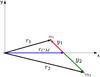
The fixed frame is centred on the Sun, the x axis is chosen in direction
of the initial centre of mass (CM) of the two asteroids and the y axis is
perpendicular to the x axis in the rotation plane of the CM. The
equations of motion for the coordinates of the first asteroid r1,
of the second one r2 and of Neptune rN are
(Whipple & Szebehely 1984): 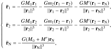 (1)where
G is the gravitational constant and M⊙,
M′, m1 and
m2 are respectively the mass of the Sun, of Neptune, of the
first asteroid and of the second one.
(1)where
G is the gravitational constant and M⊙,
M′, m1 and
m2 are respectively the mass of the Sun, of Neptune, of the
first asteroid and of the second one.
We introduce some scalings and normalisations to simplify the problem: 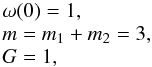 (2)where
ω(t) is the (not necessarily constant) angular mean
motion of the CM around the Sun:
(2)where
ω(t) is the (not necessarily constant) angular mean
motion of the CM around the Sun: 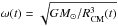 ,
RCM(t) being the radius of the centre of
mass at time t. The first normalisation defines the unit of time, the
second one, the unit of mass and the last one, the unit of length.
,
RCM(t) being the radius of the centre of
mass at time t. The first normalisation defines the unit of time, the
second one, the unit of mass and the last one, the unit of length.
In the simulations, we will need to ascertain if the two asteroids actually form a
proto-binary. With this in mind, we will introduce the Hill sphere. In our case, the Hill
sphere is the sphere centred at CM that determines the volume within which the mutual
attraction of the asteroids dominates the attraction of the Sun (see Goldreich et al. 2004; Murray &
Dermott 2000). The radius of this sphere, called the Hill sphere radius, is
defined by![Mathematical equation: \begin{equation} R_{\rm Hill}= R_{\rm CM} \sqrt[3]{\frac{m_1+m_2}{3 ~M_{\odot}}}\cdot \end{equation}](/articles/aa/full_html/2013/10/aa21137-13/aa21137-13-eq24.png) (3)With this choice of
units, the Hill sphere radius is equal to 1. So, if the distance between the potential
binary partners is smaller than 1, the two asteroids may potentially form a proto-binary.
Conversely, if the distance is larger than 1, the asteroids will revolve around the Sun
and will not form a binary.
(3)With this choice of
units, the Hill sphere radius is equal to 1. So, if the distance between the potential
binary partners is smaller than 1, the two asteroids may potentially form a proto-binary.
Conversely, if the distance is larger than 1, the asteroids will revolve around the Sun
and will not form a binary.
2.2. Initial conditions
The initial orbit of Neptune, which is Keplerian, is chosen in Keplerian coordinates and transformed afterwards to Cartesian coordinates. For the Circular-Neptune case, the initial semi-major axis is equal to 30.0940 AU and the eccentricity is zero. For the Eccentric-Neptune case, the initial semi-major axis is equal to 27.5 AU and the eccentricity is equal to 0.3. In any case, the longitude of the pericentre and the mean anomaly are chosen equal to 0. We have checked that the results are similar with a non null longitude of the pericentre or a non null mean anomaly. The initial conditions of the CM of the asteroids are also chosen in Keplerian coordinates and then transformed to Cartesian ones. The semi-major axis and eccentricity will depend on the specifics (binary in 3:2 resonance with Neptune or not). The longitude of the pericentre and the mean anomaly are equal to 0 (recall that the x axis is chosen in the direction of the initial CM).
For the initial position of the asteroids, we will consider:
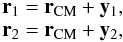 (4)where
rCM is the position vector of the CM (the initial one is already
determined) and
y1 = (x1,y1)
and
y2 = (x2,y2)
are linked by the fact that
m1y1 + m2y1 = 0.
For the initial y1 and y2, we work on a
local scale and consider that the two asteroids constitute a two body problem around their
mutual CM. With this hypothesis, the “local” energy for the first asteroid
(4)where
rCM is the position vector of the CM (the initial one is already
determined) and
y1 = (x1,y1)
and
y2 = (x2,y2)
are linked by the fact that
m1y1 + m2y1 = 0.
For the initial y1 and y2, we work on a
local scale and consider that the two asteroids constitute a two body problem around their
mutual CM. With this hypothesis, the “local” energy for the first asteroid
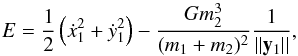 (5)remains constant. As we
are interested in binary asteroids of more or less the same mass, let us work with
m1 = m2. Then, when we use the
normalisations presented above, the energy is written
(5)remains constant. As we
are interested in binary asteroids of more or less the same mass, let us work with
m1 = m2. Then, when we use the
normalisations presented above, the energy is written 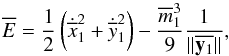 (6)where the
overbars represent normalised variables. The overbars will be omitted from now on. The
initial conditions for the asteroids are calculated in this way: first, we fix the initial
energy E. Then, as the Hill sphere is constructed for the sum of both
asteroids, x1(0) and y1(0) are
chosen between −0.5 and 0.5. We choose ẋ1(0) = 0 and
ẏ1(0) must satisfy the energy integral:
(6)where the
overbars represent normalised variables. The overbars will be omitted from now on. The
initial conditions for the asteroids are calculated in this way: first, we fix the initial
energy E. Then, as the Hill sphere is constructed for the sum of both
asteroids, x1(0) and y1(0) are
chosen between −0.5 and 0.5. We choose ẋ1(0) = 0 and
ẏ1(0) must satisfy the energy integral: 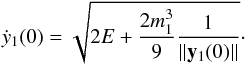 (7)Initial conditions are
real numbers only if the term under the square root is positive. If it is not the case,
the simulation is stopped. We choose in (7)
the positive sign for ẏ1(0) but in fact, the negative case
gives the same results as the positive case with
(7)Initial conditions are
real numbers only if the term under the square root is positive. If it is not the case,
the simulation is stopped. We choose in (7)
the positive sign for ẏ1(0) but in fact, the negative case
gives the same results as the positive case with  .
The MEGNO maps for example (see Sect. 2.4) will be
the same in the positive as in the negative case through an axial symmetry in
x and y and the Monte Carlo simulations (see Sect.
2.5) will not be affected by the choice of one or
the other possibility. For the second asteroid,
x2 = −x1,
y2 = −y1,
ẋ2 = 0 and
ẏ2 = −ẏ1.
.
The MEGNO maps for example (see Sect. 2.4) will be
the same in the positive as in the negative case through an axial symmetry in
x and y and the Monte Carlo simulations (see Sect.
2.5) will not be affected by the choice of one or
the other possibility. For the second asteroid,
x2 = −x1,
y2 = −y1,
ẋ2 = 0 and
ẏ2 = −ẏ1.
The simulations2 were performed using an Adams-Bashforth-Moulton 10th order predictor-corrector integrator (Hairer et al. 2008), already implemented and used in Verheylewegen et al. (2013).
The masses are fixed at 1.98892 × 1030 kg for the Sun (M⊙) and 1.02410 × 1026 kg for Neptune (M′)3. We approximate the mass of both asteroids by 2.0 × 10¹⁸ kg, similar to the primary in the 1998 WW31 system (see Veillet et al. 2002). However, the results are similar with smaller equal masses down to 2.0 × 10¹⁷ kg. This corresponds to a sphere with a diameter of about 90 km with a reasonable assumption of bulk density of 1.5 grams per cubic centimetre. This range of masses is consistent with the database of binary asteroids http://www.johnstonsarchive.net/astro/astmoontable.html.
2.3. Chaos indicators and numerical methods
The first indicator used is the surface of section (SOS, singular and plural). The SOS are computed in this way: a grid of initial conditions (with E fixed and ẋ1(0) = 0) are integrated up to a predetermined time. When the trajectory crosses the planar section ẋ1 = 0 with a positive ẏ1, the point is recorded and plotted. A trajectory tracing a solid curve is indicative of a quasi-periodic trajectory while one that fills a two-dimensional area indicates chaotic motion.
In order to distinguish between regular and chaotic orbits, we use, as a second indicator, the MEGNO map defined by Cincotta & Simó (2000). The MEGNO map is a fast chaos indicator which has proven to be reliable in a broad number of dynamical systems (Cincotta et al. 2003; Goździewski et al. 2001, 2008; Breiter et al. 2005; Compère et al. 2012; Frouard & Compère 2012). The MEGNO is a characterisation of the divergence rate of two nearby orbits and is based on the numerical integration of a tangent vector defined for the orbits. For stable orbits, the MEGNO converges towards 2 for quasi-periodic orbits and towards 0 for periodic orbits. For chaotic motion, the MEGNO increases linearily with time with a slope that is half of the Lyapunov characteristic exponent value of the orbit (Benettin et al. 1980).
In our program, the variational equations and the MEGNO differential equations of Goździewski et al. (2001) are integrated along with the equations of motion. The choice of the initial tangent vector does not influence its evolution and so this is set randomly. The computation of an orbit is stopped if its MEGNO value attains 5. On the maps, the points with a value equal to 10 correspond to scattering orbits escaping before the end of the simulation.
The last tool used is a two-dimensional Monte Carlo simulation as in Astakhov et al. (2003). A set of test asteroids is taken randomly in the Hill sphere: E is chosen randomly in [−3, −0.4] and x1(0) and y1(0) are taken randomly in [−0.5,0.5]. The bounds for E are chosen in a way that enough initial conditions are real numbers (so E is not too big) and non chaotic in the non-resonant case (so E is not too small). Indeed we need initial conditions which are a temporarily trapped binary system. The mutual orbits computed with these initial conditions are usually close to parabolic ones.
We let each system (with  ) evolve until one of the
following situations occurs: the asteroid leaves the Hill’s sphere
(| |y1|| > 0.5) or it survives for
a predetermined cut-off time (here 10 000 years). As a second step, we use these final
conditions to perform back integrations in time until again the exit of the asteroid or
the reach of a predetermined cut-off time (here, −10 000 years). The total time in
these integrations gives us the residence time of the asteroids in the Hill sphere, i.e.
the time during which the asteroids remain inside the Hill sphere. The reason for the
backwards in time integration is that when we pick random initial conditions, some of them
will escape almost immediately because they are picked “on their way out” of the Hill
sphere. By back integrating, their actual total residence time can be computed accurately.
We then plot histograms of the residence time of all the initial conditions.
) evolve until one of the
following situations occurs: the asteroid leaves the Hill’s sphere
(| |y1|| > 0.5) or it survives for
a predetermined cut-off time (here 10 000 years). As a second step, we use these final
conditions to perform back integrations in time until again the exit of the asteroid or
the reach of a predetermined cut-off time (here, −10 000 years). The total time in
these integrations gives us the residence time of the asteroids in the Hill sphere, i.e.
the time during which the asteroids remain inside the Hill sphere. The reason for the
backwards in time integration is that when we pick random initial conditions, some of them
will escape almost immediately because they are picked “on their way out” of the Hill
sphere. By back integrating, their actual total residence time can be computed accurately.
We then plot histograms of the residence time of all the initial conditions.
2.4. Surfaces of section and MEGNO maps in the planar 2 + 2 body problem
In this subsection, we present surfaces of sections (SOS) and MEGNO maps of the 2 + 2 body problem (with CM in the 3:2 resonance with Neptune or in the classical belt). In the SOS, 100 initial conditions (with x(0) ∈ [−0.5,0.5], y(0) = 0, E fixed, ẋ1(0) = 0 and ẏ1(0) as in (7)) are integrated up to 50 000 years with a step of 0.1 h. For the MEGNO maps, each point of a grid of 150 × 150 initial conditions corresponds to the MEGNO value associated to the orbit after 104 years with a step of 1 h.
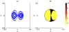 |
Fig. 1 Comparison between a) SOS and b) MEGNO maps for the planar 2 + 2 body problem for the Circular-Neptune case. The maps are done with the CM in the classical belt (R = 45 AU) and the value of the initial energy E is –1.5. |
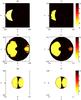 |
Fig. 2 MEGNO maps of the planar 2 + 2 body problem for the Circular-Neptune case. The maps in the left are done with the CM in the classical belt (R = 45 AU) and the ones in the right are done with the CM in the resonance (R = 39.4343 AU). The values of the initial energy E are, from top to bottom: –0.5, –0.75 and –1.5. |
Figure 1 shows a comparison between a SOS and a MEGNO map for a specific value of the energy in the 2 + 2 body problem for the Circular-Neptune case. The positive values of x of each graph correspond to prograde orbits while the negative ones correspond to retrograde orbits. As we can see, the MEGNO map shows similar characteristics to the SOS plot. We conclude that this indicator is adequate to bring out the dynamics of the orbits. The SOS, which is a graphical method, has severe restrictions when dealing with systems with more than 2 degrees of freedom. In contrast, the MEGNO indicator has proven to be a very useful tool even with more degrees of freedom (as will be the case here) (Gamboa Suárez et al. 2010; Maffione et al. 2011). In addition, MEGNO has the advantage of being able to pick out resonances and to make a clear distinction between initial conditions leading to chaotic orbits. Also, “forbidden” regions of phase space are easier to demarcate using MEGNO: in the MEGNO maps, unphysical (forbidden) initial conditions are plotted in white.
Now, we come back to our central question: is there a difference in the stability of orbits in the 3:2 resonance with Neptune and outside the resonance. To investigate that point, we construct MEGNO maps of the 2 + 2 body problem with the centre of mass of the asteroids in the resonance or in the classical belt. We will first look at the Circular-Neptune case. In the resonance, the radius R is equal to 39.4343 AU and we choose to take R = 45 AU to analyse what happens outside the resonance. The choice is motivated by the fact that, in this case, the two asteroids are in the classical Kuiper belt which means that they are not influenced by any resonance with Neptune. However, all our results are unchanged if we take for example R = 40 AU instead of R = 45 AU.
The results are presented in Fig. 2. We can first analyse the maps outside the resonance (i.e. the maps in the left-most column): for the prograde orbits, the mapping is very regular for low values of E (map (e)). Then some chaotic and scattering zones appear when E increases (maps (c)) leading to a mainly scattering map for higher E (maps (a)). In fact, up to E ~ −0.7, no prograde orbits are regular. The retrograde orbits are not as much influenced by E as are the prograde orbits.
If we compare now the maps outside and in the resonance, we see the influence of the resonance on some orbits, especially for E = −0.75. The resonance induces some extremely stable orbits (with a MEGNO value of 0) but mainly chaotic and scattering ones. For E around −0.75, the prograde stable zones are totally destroyed. This leads us to think that a random initial binary will have less chance to be created in the resonant case.
The same figure can be drawn for the Eccentric-Neptune case. In this case, the radius R is equal to 36.0352 AU in the resonance and to 40 AU in the classical belt. The results are shown in Fig. 3. The maps do not show many differences according to the location of the centre of mass. This is then not sufficient to explain the lack of binaries.
Percentage of binaries in each residence times category for all the cases studied in this article.
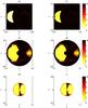 |
Fig. 3 MEGNO maps of the planar 2 + 2 body problem for the Eccentric-Neptune case. The maps in the left are done with the CM in the classical belt (R = 40 AU) and the ones in the right are done with the CM in the resonance (R = 36.0352 AU). The values of the initial energy E are from top to bottom: –0.5, –0.75 and –1.5. |
We will now compute residence times to see if these calculations confirm our assumptions.
2.5. Residence times in the planar circular 2 + 2 body problem
Histograms of residence times in the resonance and in the classical belt (for one hundred thousand initial conditions) are presented in Fig. 4 for the Circular-Neptune case and in Fig. 5 for the Eccentric-Neptune case. The orbits are binned using a logarithmic scale. The asteroids fall mainly into three categories: binaries which exit the Hill sphere in less than 2000 years, binaires staying coupled between 2000 and 20 000 years and asteroids which remain inside the Hill sphere for 20 000 years or longer (in red). The last category corresponds mainly to orbits in a stable zone which were not (and will not be) disrupted, so they are not captured orbits (that is why this bin is drawn in red). The second category represent only a few number of orbit according to the total number of initial conditions. So mainly all the captured orbits fall in the first category, which means that they stay coupled for less than 2000 years. The distribution of the number of orbits in the three categories is given in Table 1. These results are in agreement with the MEGNO maps: if we simplify, for the Circular-Neptune case, some stable orbits (so in the third category) in the classical belt become chaotic (in the second category) or scattering (in the first category) in the resonance. However, these changes are really weak. For the Eccentric-Neptune case, there is even less differences. This prompted us to introduce another influence of the resonance in the model: an initial non-null eccentricity for the CM.
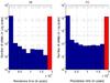 |
Fig. 4 Distribution of residence times (in Log scale) of 100 000 asteroids in the Hill sphere of the CM (with a null eccentricity) in the planar 2 + 2 body problem for the Circular-Neptune case. In a), the CM is in the classical belt (R = 45 AU) and in b), the CM is in the resonance (R = 39.4343 AU). These histograms are linked to the MEGNO maps of Fig. 2. |
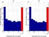 |
Fig. 5 Distribution of residence times (in Log scale) of 100 000 asteroids in the Hill sphere of the CM (with a null eccentricity) in the planar 2 + 2 body problem for the Eccentric-Neptune case. In a) the CM is in the classical belt (R = 40 AU) and in b) the CM is in the resonance (R = 36.0352 AU). These histograms are linked to the MEGNO maps of Fig. 3. |
3. The 2 + 2 body problem: the planar eccentric case
Mean-motion resonances between a planet and an asteroid usually have the effect of increasing the eccentricity of the asteroid. This is confirmed for the 3:2 resonance with Neptune in the Kuiper Belt population, as shown in Fig. 6. Indeed, this figure presents the eccentricities (versus semi-major axes) of the trans-Neptunian objects present in the database of the Minor Planet Center. We can clearly see that, in the resonance (at approximately 39.4 AU), the eccentricities are mainly concentrated in the range [0.1; 0.35]. This is also confirmed for example, in Malhotra et al. (2000) and in Hahn & Malhotra (2005). These articles clearly show larger eccentricities for the objects in mean motion resonance with Neptune and especially eccentricities up to 0.35 for the 3:2 resonance.
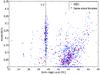 |
Fig. 6 Distribution of eccentricities according to the semi-major axes of the currently known trans-Neptunian objects. The position of the 3:2 resonance and the locations of known, roughly same-sized trans-Neptunian binaries. Data from the Minor Planet Center and from the database http://www.johnstonsarchive.net/astro/astmoontable.html |
3.1. MEGNO maps in the planar eccentric case
Assuming eccentricities comparable to those observed for the Plutinos, we integrate the equations of motion and compute MEGNO maps. Because we are looking at the last stage of the migration of Neptune, we can assume that the growth of the eccentricity of objects captured into resonance is almost finished. MEGNO maps for two different values of E and for initial eccentricities of the CM of 0, 0.1 and 0.3 are compared in Figs. 7 and 8 for the Circular-Neptune case and the Eccentric-Neptune case.
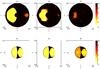 |
Fig. 7 MEGNO maps of the 2 + 2 body problem with the CM in the resonance (R = 39.4343 AU) for the Circular-Neptune case. The value of the initial energy E is –0.75 for the top frames and –1.5 for the bottom frames. The initial eccentricity of the CM is, from left to right: 0, 0.1 and 0.3. |
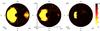 |
Fig. 8 MEGNO maps of the 2 + 2 body problem with the CM in the resonance (R = 36.0352 AU) for the Eccentric-Neptune case. The value of the initial energy E is –0.75. The initial eccentricity of the CM is, from left to right: 0, 0.1 and 0.3. |
With an initial eccentricity of 0.3, almost all the orbits are scattering or chaotic, especially for the Circular-Neptune case. The KAM islands are totally destroyed for both prograde and retrograde orbits suggesting that few binary asteroids can be created in the 3:2 resonance if the eccentricity of the centre of mass is large.
Note that for stable orbits, the eccentricity will stay close to its initial value during the integrations. For example, the variation of an initial eccentricity of 0.1 is about 0.012 with a period of 9000 years.
The scattering behaviour of the orbits mainly comes from the eccentricity of the CM and not from the direct influence of the resonance. This is shown in Fig. 9 which shows the same MEGNO maps as Fig. 7 but with the CM outside the resonance. So, few binaries can be created with a high eccentricity. Obviously, eccentric asteroids are also present in other regions of the Kuiper Belt but in smaller numbers (see Fig. 6). The classical belt is mainly composed of asteroids on nearly circular orbits. In fact, we can see in Fig. 6 that the classical belt contains only a small number of same-sized binaries with a large eccentricity (proportionally to the number of detected binaries). On the other hand, mainly all the asteroids in the 3:2 resonance have large eccentricities. These results suggest that the proportion of binary asteroids created in the 3:2 resonance will be lower than in the classical belt.
3.2. Residence times in the planar eccentric case
We now compute histograms of the residence times of binary asteroids with an initially eccentric CM. For the Circular-Neptune case, the results are shown in Fig. 10 for the non-resonant and non-eccentric case (in the left) and for the resonant one with an initial eccentricity of the CM of 0.3 (in the right). Similar graphs are shown in Fig. 11 for the Eccentric-Neptune case. The distribution of the number of orbits in the three categories is also given in Table 1.
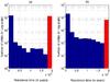 |
Fig. 10 Distribution of residence times (in Log scale) of 100 000 asteroids in the Hill sphere of the CM in the planar 2 + 2 body problem for the Circular-Neptune case. In a) the CM is in the classical belt (R = 45 AU) and with a null eccentricity and in b) the CM is in the resonance (R = 39.4343 AU) and the initial eccentricity of the CM is 0.3. These histograms are linked to the MEGNO maps of Fig. 7. |
 |
Fig. 11 Distribution of residence times (in Log scale) of 100 000 asteroids in the Hill sphere of the CM in the planar 2 + 2 body problem for the Eccentric-Neptune case. In a), the CM is in the classical belt (R = 40 AU) and with a null eccentricity and in b), the CM is in the resonance (R = 36.0352 AU) and the initial eccentricity of the CM is 0.3. These histograms are linked to the MEGNO maps of Fig. 8. |
The number of binary asteroids that form proto-binaries lasting more than 20 000 years in the resonant eccentric case is about half the number in the non-resonant circular case (the numbers of orbits are given in Log scale in the histograms). This means that the stable zones are really smaller in the resonant-eccentric case. This strengthens the conclusion about the MEGNO maps: almost all the stable zones in the non-resonant circular case became scattering or chaotic in the resonant eccentric case. This means that the number of binary asteroids in the first and in the second category grows in the resonant eccentric case. However, the number of binaries in the second category remains a small fraction of the total number of test particles. These results support therefore the idea that there is much less stable zones for binary asteroids in the 3:2 resonance than in the classical belt.
4. The 2 + 2 body problem: the non-planar eccentric case
We can also check the results in the non-planar 2 + 2 body problem. Figure 12 shows the inclinations (versus semi-major axes) of the trans-Neptunian objects present in the database of the Minor Planet Center. We see that the objects in the 3:2 resonance with Neptune (at approximately 39.4 AU) cover a large range of inclinations. In order to understand the affect of inclination, we include the third dimension and choose a random initial inclination for the heliocentric CM (between 0° and 60°) also for the mutual orbit (also between 0° and 60°). The results are presented in Fig. 13 and in Table 1 for the Circular-Neptune case in both cases: the non-resonant non-eccentric case and the resonant eccentric one. The results for the Eccentric-Neptune case are similar.
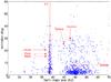 |
Fig. 12 Same as Fig. 6 but for the distribution of inclinations according to the semi-major axes of the currently known trans-Neptunian objects. |
The effect of the inclination is to decrease the number of long-lived binaries in both cases. Nevertheless, the ratio of binaries coupled for 20 000 years or more in the resonant and in the non-resonant case is more or less the same as in the planar 2 + 2 body problem. We can then say that the conclusions drawn in the planar case are still valid in the non-planar one.
5. Conclusions
The goal of this article was to provide insight into the scarcity of binary asteroids among the Plutinos. We assumed that binary formation occurred in situ (within the present day Kuiper belt) when Neptune’s eccentricity was damping (according to the Nice model). Using the 2 + 2 body approximation of Whipple & Szebehely (1984) and Whipple & White (1985), we took into account the fact that the 3:2 resonance increases the eccentricity of the centre of mass of the asteroids. We performed numerical integrations of the motion of test particles inside their common Hill sphere to determine whether or not they formed a binary. We plotted MEGNO maps and histograms of the residence time of these particles inside and outside the resonant zone for two different periods of formation (called here the Circular-Neptune and the Eccentric-Neptune cases). The MEGNO maps showed, for both epochs, that the stable zones present in the non-resonant case are almost totally destroyed for both prograde and retrograde orbits in the eccentric resonant case. This means that two asteroids cannot easily form a stable and long-lived binary. Furthermore, the histograms of residence times showed that far fewer binaries can stay coupled for more than 20 000 years in the Plutinos region.
Our results indicate that a pair of asteroids in the resonance has less chance to form a binary than a corresponding couple exterior to the resonance. Moreover the higher the eccentricity of their CM, the smaller the probability of binary capture. This means that objects formed or trapped for very long times in the resonances will not produce many binaries. So the small number of binaries observed in the 3:2 resonance are probably very robust old binaries, which avoided close encounters with Neptune and ended up trapped in the resonance, only after Neptune’s eccentricity was damped.
A video of the talk can be found here: https://webcast.stsci.edu/webcast/detail.xhtml?talkid=1912&parent=1. Here we investigate possible reasons for the lack of binary asteroids among the Plutinos.
The computations were performed on an HPC cluster at the Interuniversity Scientific Computing Facility center (iSCF – http://www.iscf.be) located at the University of Namur (Belgium).
Acknowledgments
The authors thank the anonymous reviewer for very constructive and insightful comments on an earlier version of the paper. This research used resources of the Interuniversity Scientific Computing Facility located at the University of Namur, Belgium, which is supported by the F.R.S.-FNRS under convention No. 2.4617.07. This work was partially supported by a grant from the US National Science Foundation to Utah State University (Award No. 1300504).
References
- Astakhov, S. A., & Farrelly, D. 2004, MNRAS, 354, 971 [NASA ADS] [CrossRef] [Google Scholar]
- Astakhov, S. A., Burbanks, A. D., Wiggins, S., & Farrelly, D. 2003, Nature, 423, 264 [NASA ADS] [CrossRef] [Google Scholar]
- Astakhov, S. A., Lee, E. A., & Farrelly, D. 2005, MNRAS, 360, 401 [NASA ADS] [CrossRef] [Google Scholar]
- Benettin, G., Galgani, L., Giorgilli, A., & Strelcyn, J.-M. 1980, Meccanica, 15, 9 [NASA ADS] [CrossRef] [Google Scholar]
- Breiter, S., Melendo, B., Bartczak, P., & Wytrzyszczak, I. 2005, A&A, 437, 753 [NASA ADS] [CrossRef] [EDP Sciences] [Google Scholar]
- Cincotta, P. M., & Simó, C. 2000, A&AS, 147, 205 [NASA ADS] [CrossRef] [EDP Sciences] [Google Scholar]
- Cincotta, P. M., Giordano, C. M., & Simó, C. 2003, Phys. D, 182, 151 [NASA ADS] [CrossRef] [Google Scholar]
- Compère, A., Lemaître, A., & Delsate, N. 2012, Celest. Mech. Dyn. Astron., 112, 75 [NASA ADS] [CrossRef] [Google Scholar]
- Farrelly, D., Hestroffer, D., Astakhov, S. A., et al. 2006, BAAS, 38, 1300 [NASA ADS] [Google Scholar]
- Frouard, J., & Compère, A. 2012, Icarus, 220, 149 [NASA ADS] [CrossRef] [Google Scholar]
- Funato, Y., Makino, J., Hut, P., Kokubo, E., & Kinoshita, D. 2004, Nature, 427, 518 [NASA ADS] [CrossRef] [Google Scholar]
- Gamboa Suárez, A., Hestroffer, D., & Farrelly, D. 2010, Celest. Mech. Dyn. Astron., 106, 245 [NASA ADS] [CrossRef] [Google Scholar]
- Goldreich, P., Lithwick, Y., & Sari, R. 2002, Nature, 420, 643 [NASA ADS] [CrossRef] [PubMed] [Google Scholar]
- Goldreich, P., Lithwick, Y., & Sari, R. 2004, ARA&A, 42, 549 [NASA ADS] [CrossRef] [Google Scholar]
- Gomes, R. S. 2003, Icarus, 161, 404 [Google Scholar]
- Gomes, R., Levison, H. F., Tsiganis, K., & Morbidelli, A. 2005, Nature, 435, 466 [NASA ADS] [CrossRef] [PubMed] [Google Scholar]
- Goździewski, K., Bois, E., Maciejewski, A. J., & Kiseleva-Eggleton, L. 2001, A&A, 378, 569 [NASA ADS] [CrossRef] [EDP Sciences] [Google Scholar]
- Goździewski, K., Breiter, S., & Borczyk, W. 2008, MNRAS, 383, 989 [NASA ADS] [CrossRef] [Google Scholar]
- Grundy, W. M., Noll, K. S., Nimmo, F., et al. 2011, Icarus, 213, 678 [NASA ADS] [CrossRef] [Google Scholar]
- Hahn, J. M., & Malhotra, R. 2005, AJ, 130, 2392 [NASA ADS] [CrossRef] [Google Scholar]
- Hairer, E., Nørsett, S., & Wanner, G. 2008, Solving Ordinary Differential Equations I: Nonstiff Problems (Springer) [Google Scholar]
- Kominami, J. D., Makino, J., & Daisaka, H. 2011, PASJ, 63, 1331 [NASA ADS] [Google Scholar]
- Lee, E. A., Astakhov, S. A., & Farrelly, D. 2007, MNRAS, 379, 229 [NASA ADS] [CrossRef] [Google Scholar]
- Levison, H. F., & Morbidelli, A. 2003, Nature, 426, 419 [NASA ADS] [CrossRef] [PubMed] [Google Scholar]
- Levison, H. F., Morbidelli, A., Van Laerhoven, C., Gomes, R., & Tsiganis, K. 2008, Icarus, 196, 258 [NASA ADS] [CrossRef] [Google Scholar]
- Maffione, N. P., Darriba, L. A., Cincotta, P. M., & Giordano, C. M. 2011, Celest. Mech. Dyn. Astron., 111, 285 [NASA ADS] [CrossRef] [Google Scholar]
- Malhotra, R. 1995, AJ, 110, 420 [NASA ADS] [CrossRef] [Google Scholar]
- Malhotra, R., Duncan, M. J., & Levison, H. F. 2000, Protostars and Planets IV, 1231 [Google Scholar]
- Morbidelli, A., Levison, H. F., Tsiganis, K., & Gomes, R. 2005, Nature, 435, 462 [NASA ADS] [CrossRef] [PubMed] [Google Scholar]
- Murray, C. D., & Dermott, S. F. 2000, Solar System Dynamics (CUP) [Google Scholar]
- Murray-Clay, R. A., & Schlichting, H. E. 2011, ApJ, 730, 132 [NASA ADS] [CrossRef] [Google Scholar]
- Nesvorný, D., Youdin, A. N., & Richardson, D. C. 2010, AJ, 140, 785 [NASA ADS] [CrossRef] [Google Scholar]
- Noll, K. S. 2003, Earth Moon and Planets, 92, 395 [NASA ADS] [CrossRef] [Google Scholar]
- Noll, K. S., Stephens, D. C., Grundy, W. M., & Griffin, I. 2004, Icarus, 172, 402 [NASA ADS] [CrossRef] [Google Scholar]
- Noll, K. S., Grundy, W. M., Chiang, E. I., Margot, J.-L., & Kern, S. D. 2008, Binaries in the Kuiper Belt, eds. M. A. Barucci, H. Boehnhardt, D. P. Cruikshank, A. Morbidelli, & R. Dotson, 345 [Google Scholar]
- Parker, A. H., & Kavelaars, J. J. 2010, ApJ, 722, L204 [NASA ADS] [CrossRef] [Google Scholar]
- Porter, S. B., & Grundy, W. M. 2012, Icarus, 220, 947 [NASA ADS] [CrossRef] [Google Scholar]
- Sheppard, S. S., Ragozine, D., & Trujillo, C. 2012, AJ, 143, 58 [NASA ADS] [CrossRef] [Google Scholar]
- Tsiganis, K., Gomes, R., Morbidelli, A., & Levison, H. F. 2005, Nature, 435, 459 [NASA ADS] [CrossRef] [PubMed] [Google Scholar]
- Veillet, C., Parker, J. W., Griffin, I., et al. 2002, Nature, 416, 711 [NASA ADS] [CrossRef] [Google Scholar]
- Verheylewegen, E., Noyelles, B., & Lemaitre, A. 2013, MNRAS [Google Scholar]
- Weidenschilling, S. J. 2002, Icarus, 160, 212 [NASA ADS] [CrossRef] [Google Scholar]
- Whipple, A. L., & Szebehely, V. 1984, Celestial Mechanics, 32, 137 [NASA ADS] [CrossRef] [Google Scholar]
- Whipple, A. L., & White, L. K. 1985, Celestial Mechanics, 35, 95 [NASA ADS] [CrossRef] [Google Scholar]
All Tables
Percentage of binaries in each residence times category for all the cases studied in this article.
All Figures
|
Fig. 1 Comparison between a) SOS and b) MEGNO maps for the planar 2 + 2 body problem for the Circular-Neptune case. The maps are done with the CM in the classical belt (R = 45 AU) and the value of the initial energy E is –1.5. |
| In the text | |
|
Fig. 2 MEGNO maps of the planar 2 + 2 body problem for the Circular-Neptune case. The maps in the left are done with the CM in the classical belt (R = 45 AU) and the ones in the right are done with the CM in the resonance (R = 39.4343 AU). The values of the initial energy E are, from top to bottom: –0.5, –0.75 and –1.5. |
| In the text | |
|
Fig. 3 MEGNO maps of the planar 2 + 2 body problem for the Eccentric-Neptune case. The maps in the left are done with the CM in the classical belt (R = 40 AU) and the ones in the right are done with the CM in the resonance (R = 36.0352 AU). The values of the initial energy E are from top to bottom: –0.5, –0.75 and –1.5. |
| In the text | |
|
Fig. 4 Distribution of residence times (in Log scale) of 100 000 asteroids in the Hill sphere of the CM (with a null eccentricity) in the planar 2 + 2 body problem for the Circular-Neptune case. In a), the CM is in the classical belt (R = 45 AU) and in b), the CM is in the resonance (R = 39.4343 AU). These histograms are linked to the MEGNO maps of Fig. 2. |
| In the text | |
|
Fig. 5 Distribution of residence times (in Log scale) of 100 000 asteroids in the Hill sphere of the CM (with a null eccentricity) in the planar 2 + 2 body problem for the Eccentric-Neptune case. In a) the CM is in the classical belt (R = 40 AU) and in b) the CM is in the resonance (R = 36.0352 AU). These histograms are linked to the MEGNO maps of Fig. 3. |
| In the text | |
|
Fig. 6 Distribution of eccentricities according to the semi-major axes of the currently known trans-Neptunian objects. The position of the 3:2 resonance and the locations of known, roughly same-sized trans-Neptunian binaries. Data from the Minor Planet Center and from the database http://www.johnstonsarchive.net/astro/astmoontable.html |
| In the text | |
|
Fig. 7 MEGNO maps of the 2 + 2 body problem with the CM in the resonance (R = 39.4343 AU) for the Circular-Neptune case. The value of the initial energy E is –0.75 for the top frames and –1.5 for the bottom frames. The initial eccentricity of the CM is, from left to right: 0, 0.1 and 0.3. |
| In the text | |
|
Fig. 8 MEGNO maps of the 2 + 2 body problem with the CM in the resonance (R = 36.0352 AU) for the Eccentric-Neptune case. The value of the initial energy E is –0.75. The initial eccentricity of the CM is, from left to right: 0, 0.1 and 0.3. |
| In the text | |
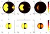 |
Fig. 9 Same as Fig. 7 but with the CM in the classical belt (R = 45 AU). |
| In the text | |
|
Fig. 10 Distribution of residence times (in Log scale) of 100 000 asteroids in the Hill sphere of the CM in the planar 2 + 2 body problem for the Circular-Neptune case. In a) the CM is in the classical belt (R = 45 AU) and with a null eccentricity and in b) the CM is in the resonance (R = 39.4343 AU) and the initial eccentricity of the CM is 0.3. These histograms are linked to the MEGNO maps of Fig. 7. |
| In the text | |
|
Fig. 11 Distribution of residence times (in Log scale) of 100 000 asteroids in the Hill sphere of the CM in the planar 2 + 2 body problem for the Eccentric-Neptune case. In a), the CM is in the classical belt (R = 40 AU) and with a null eccentricity and in b), the CM is in the resonance (R = 36.0352 AU) and the initial eccentricity of the CM is 0.3. These histograms are linked to the MEGNO maps of Fig. 8. |
| In the text | |
|
Fig. 12 Same as Fig. 6 but for the distribution of inclinations according to the semi-major axes of the currently known trans-Neptunian objects. |
| In the text | |
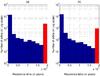 |
Fig. 13 Same as Fig. 10 but in the non-planar 2 + 2 bodies. |
| In the text | |
Current usage metrics show cumulative count of Article Views (full-text article views including HTML views, PDF and ePub downloads, according to the available data) and Abstracts Views on Vision4Press platform.
Data correspond to usage on the plateform after 2015. The current usage metrics is available 48-96 hours after online publication and is updated daily on week days.
Initial download of the metrics may take a while.