© ESO, 2013

1. Introduction

The dependence of the luminosity distance d_L(z) on the redshift z is a key formula in cosmology (Carroll et al. 1992). It is given by three independent cosmological parameters: by two omega-parameters Ω_M, Ω_Λ, and by the Hubble constant H₀. Its relation to the so-called proper-motion distance is given by d_PM(z)(1 + z) = d_L(z) (Weinberg 1972).

One has (Carroll et al. 1992)

$\begin{array}{ccc}& & {\mathit{d}}_{\mathrm{PM}}\mathrm{\left(}\mathit{z}\mathrm{\right)}\mathrm{=}\frac{\mathit{c}}{{\mathit{H}}_{\mathrm{0}}\sqrt{\mathrm{\left|}{\mathrm{\Omega }}_{\mathit{k}}\mathrm{\right|}}}\\ & & \mathrm{\times }\mathrm{sinn}\begin{array}{c}\mathrm{⎧}\\ \mathrm{⎪}\\ \mathrm{⎪}\\ \mathrm{⎨}\\ \mathrm{⎪}\\ \mathrm{⎪}\\ \mathrm{⎩}\end{array}\sqrt{\mathrm{\left|}{\mathrm{\Omega }}_{\mathit{k}}\mathrm{\right|}}{\mathrm{\int }}_{\mathrm{0}}^{\mathit{z}}\frac{\mathrm{d}{\mathit{z}}^{\mathrm{\prime }}}{\sqrt{\mathrm{(}\mathrm{1}\mathrm{+}{\mathit{z}}^{\mathrm{\prime }}{\mathrm{)}}^{\mathrm{2}}\mathrm{(}\mathrm{1}\mathrm{+}{\mathrm{\Omega }}_{\mathrm{M}}{\mathit{z}}^{\mathrm{\prime }}\mathrm{)}\mathrm{-}{\mathit{z}}^{\mathrm{\prime }}\mathrm{(}\mathrm{2}\mathrm{+}{\mathit{z}}^{\mathrm{\prime }}\mathrm{)}{\mathrm{\Omega }}_{\mathrm{\Lambda }}}}\begin{array}{c}\mathrm{⎫}\\ \mathrm{⎪}\\ \mathrm{⎪}\\ \mathrm{⎬}\\ \mathrm{⎪}\\ \mathrm{⎪}\\ \mathrm{⎭}\end{array}\mathit{.}\end{array}$(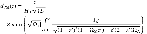1)

In this equation c is the speed of light in vacuum, and it holds Ω_k + Ω_M + Ω_Λ = 1. The notation “sinn” means the standard function sinh for Ω_k > 0, and sin for Ω_k < 0, respectively. If Ω_k = 0, then one simply has an integration: 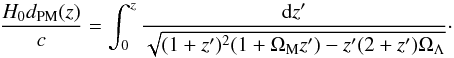$\frac{{\mathit{H}}_{\mathrm{0}}{\mathit{d}}_{\mathrm{PM}}\mathrm{\left(}\mathit{z}\mathrm{\right)}}{\mathit{c}}\mathrm{=}{\mathrm{\int }}_{\mathrm{0}}^{\mathit{z}}\frac{\mathrm{d}{\mathit{z}}^{\mathrm{\prime }}}{\sqrt{\mathrm{(}\mathrm{1}\mathrm{+}{\mathit{z}}^{\mathrm{\prime }}{\mathrm{)}}^{\mathrm{2}}\mathrm{(}\mathrm{1}\mathrm{+}{\mathrm{\Omega }}_{\mathrm{M}}{\mathit{z}}^{\mathrm{\prime }}\mathrm{)}\mathrm{-}{\mathit{z}}^{\mathrm{\prime }}\mathrm{(}\mathrm{2}\mathrm{+}{\mathit{z}}^{\mathrm{\prime }}\mathrm{)}{\mathrm{\Omega }}_{\mathrm{\Lambda }}}}\mathrm{·}$(2)In addition, from the physical point of view, in both equations it must be Ω_M > 0. (The case Ω_M = 0 can serve as a limit, but Ω_M < 0 is fully unphysical.) On the other hand, Ω_Λ can have both signs, but the observations of the past two decades strongly disfavour negative values (see, e.g., Perrett et al. 2012, and references therein).

In the special case of Ω_Λ = 0, the integral in Eq. (1) can be given by the so-called Mattig-formula (Mattig 1958) for any Ω_M > 0. The formula can then easily be used in cosmological applications (see, e.g., Mészáros 2002). For Ω_Λ ≠ 0 the integral in Eqs. (1), (2) is usually solved numerically¹.

In this note we show that the integral on the right-hand side of Eq. (2) can be solved analytically also for Ω_Λ ≠ 0.

2. Integration

We rewrite the right-hand side of Eq.(2) into the form 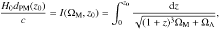$\frac{{\mathit{H}}_{\mathrm{0}}{\mathit{d}}_{\mathrm{PM}}\mathrm{\left(}{\mathit{z}}_{\mathrm{0}}\mathrm{\right)}}{\mathit{c}}\mathrm{=}\mathit{I}\mathrm{\left(}{\mathrm{\Omega }}_{\mathrm{M}}\mathit{,}{\mathit{z}}_{\mathrm{0}}\mathrm{\right)}\mathrm{=}{\mathrm{\int }}_{\mathrm{0}}^{{\mathit{z}}_{\mathrm{0}}}\frac{\mathrm{d}\mathit{z}}{\sqrt{\mathrm{(}\mathrm{1}\mathrm{+}\mathit{z}{\mathrm{)}}^{\mathrm{3}}{\mathrm{\Omega }}_{\mathrm{M}}\mathrm{+}{\mathrm{\Omega }}_{\mathrm{\Lambda }}}}\mathit{,}$(3)where z ≥ 0, Ω_M > 0 and Ω_M + Ω_Λ = 1. Introducing the substitution x = (1 + z)^-1, we obtain 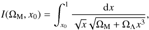$\mathit{I}\mathrm{\left(}{\mathrm{\Omega }}_{\mathrm{M}}\mathit{,}{\mathit{x}}_{\mathrm{0}}\mathrm{\right)}\mathrm{=}{\mathrm{\int }}_{{\mathit{x}}_{\mathrm{0}}}^{\mathrm{1}}\frac{\mathrm{d}\mathit{x}}{\sqrt{\mathit{x}}\sqrt{{\mathrm{\Omega }}_{\mathrm{M}}\mathrm{+}{\mathrm{\Omega }}_{\mathrm{\Lambda }}{\mathit{x}}^{\mathrm{3}}}}\mathit{,}$(4)where 0 < x₀ = (1 + z₀)^-1 ≤ 1.

In this section we consider only the case Ω_M < 1, i.e. Ω_Λ = 1 − Ω_M > 0. Introducing a further substitution y = (Ω_Λ/Ω_M)^1/3x, we obtain 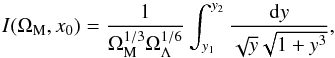$\mathit{I}\mathrm{\left(}{\mathrm{\Omega }}_{\mathrm{M}}\mathit{,}{\mathit{x}}_{\mathrm{0}}\mathrm{\right)}\mathrm{=}\frac{\mathrm{1}}{{\mathrm{\Omega }}_{\mathrm{M}}^{\mathrm{1}\mathit{/}\mathrm{3}}{\mathrm{\Omega }}_{\mathrm{\Lambda }}^{\mathrm{1}\mathit{/}\mathrm{6}}}{\mathrm{\int }}_{{\mathit{y}}_{\mathrm{1}}}^{{\mathit{y}}_{\mathrm{2}}}\frac{\mathrm{d}\mathit{y}}{\sqrt{\mathit{y}}\sqrt{\mathrm{1}\mathrm{+}{\mathit{y}}^{\mathrm{3}}}}\mathit{,}$(5)where y₁ = (Ω_Λ/Ω_M)^1/3x₀ and y₂ = (Ω_Λ/Ω_M)^1/3. The two limits are non-negative with y₁ ≤ y₂.

We aim to find the primitive function for 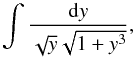$\mathrm{\int }\frac{\mathrm{d}\mathit{y}}{\sqrt{\mathit{y}}\sqrt{\mathrm{1}\mathrm{+}{\mathit{y}}^{\mathrm{3}}}}\mathit{,}$(6)where y ≥ 0. The following substitution helps: 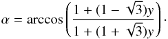$\mathit{\alpha }\mathrm{=}\arccos \left(\frac{\mathrm{1}\mathrm{+}\mathrm{(}\mathrm{1}\mathrm{-}\sqrt{\mathrm{3}}\mathrm{)}\mathit{y}}{\mathrm{1}\mathrm{+}\mathrm{(}\mathrm{1}\mathrm{+}\sqrt{\mathrm{3}}\mathrm{)}\mathit{y}}\right)\mathrm{·}$(7)There is a one-to-one correspondence between α and y. For y = 0 one has α = 0, and for y → ∞ one has ${\mathit{\alpha }}_{\mathrm{\infty }}\mathrm{\to }\arccos \mathrm{\left(}\mathrm{\right(}\mathrm{1}\mathrm{-}\sqrt{\mathrm{3}}\mathrm{)}\mathit{/}\mathrm{(}\mathrm{1}\mathrm{+}\sqrt{\mathrm{3}}\mathrm{\left)}\mathrm{\right)}$, i.e. α_∞ = 105.54°. If y increases in the interval [0,∞), α is also increasing in the interval [0,α_∞). Hence, this substitution is well-defined. Conversely, one obtains 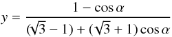$\mathit{y}\mathrm{=}\frac{\mathrm{1}\mathrm{-}\cos \mathit{\alpha }}{\mathrm{(}\sqrt{\mathrm{3}}\mathrm{-}\mathrm{1}\mathrm{)}\mathrm{+}\mathrm{(}\sqrt{\mathrm{3}}\mathrm{+}\mathrm{1}\mathrm{)}\cos \mathit{\alpha }}$(8)and $\mathrm{d}\mathit{y}\mathrm{=}\frac{\mathrm{2}\sqrt{\mathrm{3}}\sin \mathit{\alpha }\mathrm{d}\mathit{\alpha }}{\mathrm{\left[}\sqrt{\mathrm{3}}\mathrm{\right(}\mathrm{1}\mathrm{+}\cos \mathit{\alpha }\mathrm{)}\mathrm{-}\mathrm{(}\mathrm{1}\mathrm{-}\cos \mathit{\alpha }\mathrm{)}{\mathrm{]}}^{\mathrm{2}}}\mathrm{·}$(9)Using these two formulas, we curiously obtain $\frac{\mathrm{d}\mathit{y}}{\sqrt{\mathit{y}}\sqrt{\mathrm{1}\mathrm{+}{\mathit{y}}^{\mathrm{3}}}}\mathrm{=}\frac{\mathrm{d}\mathit{\alpha }}{{\mathrm{3}}^{\mathrm{1}\mathit{/}\mathrm{4}}\sqrt{\mathrm{1}\mathrm{-}\frac{\mathrm{2}\mathrm{+}\sqrt{\mathrm{3}}}{\mathrm{4}}{\sin }^{\mathrm{2}}\mathit{\alpha }}}\mathrm{·}$(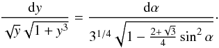10)The right-hand side of Eq. (10) is the function in the elliptic integral of the first kind (Gradshteyn et al. 2007) with 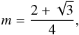$\mathit{m}\mathrm{=}\frac{\mathrm{2}\mathrm{+}\sqrt{\mathrm{3}}}{\mathrm{4}}\mathit{,}$(11)where 0 < m < 1, as it should be in an elliptic integral.

To calculate the definite integral 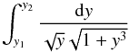${\mathrm{\int }}_{{\mathit{y}}_{\mathrm{1}}}^{{\mathit{y}}_{\mathrm{2}}}\frac{\mathrm{d}\mathit{y}}{\sqrt{\mathit{y}}\sqrt{\mathrm{1}\mathrm{+}{\mathit{y}}^{\mathrm{3}}}}$(12)in Eq. (5) for non-negative y₁ ≤ y₂, one can write 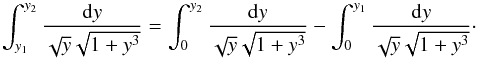${\mathrm{\int }}_{{\mathit{y}}_{\mathrm{1}}}^{{\mathit{y}}_{\mathrm{2}}}\frac{\mathrm{d}\mathit{y}}{\sqrt{\mathit{y}}\sqrt{\mathrm{1}\mathrm{+}{\mathit{y}}^{\mathrm{3}}}}\mathrm{=}{\mathrm{\int }}_{\mathrm{0}}^{{\mathit{y}}_{\mathrm{2}}}\frac{\mathrm{d}\mathit{y}}{\sqrt{\mathit{y}}\sqrt{\mathrm{1}\mathrm{+}{\mathit{y}}^{\mathrm{3}}}}\mathrm{-}{\mathrm{\int }}_{\mathrm{0}}^{{\mathit{y}}_{\mathrm{1}}}\frac{\mathrm{d}\mathit{y}}{\sqrt{\mathit{y}}\sqrt{\mathrm{1}\mathrm{+}{\mathit{y}}^{\mathrm{3}}}}\mathrm{·}$(13)After this one should use the formula with α from Eq. (10) and determine the integration limits in variable α. The substitution from Eq. (7) gives for y = 0 the value α = 0. This means

that – using α – the lower limits in both definite integrals are zeros. The upper limits from y₁ and y₂, respectively, are also calculable analytically and unambiguously from Eq. (7) via the arccos function. One obtains α₁ and α₂, respectively, as upper limits in the integrals. It must be α₂ > α₁. One should only clarify that, of course, if it were α₂ from the interval (π/2,α_∞), then the first elliptic integral itself should be given by a sum of two integrals: in one integral the limits should be 0 and π/2, and in the second one the limits should be (π − α₂) and π/2. Both integrals must give positive values. If it were also α₁ > π/2, then one should proceed similarly in the second integral, too. In any case, the integral I(Ω_M,x₀) is easily obtainable from standard elliptic integrals of the first kind.

3. Remarks

The integral in Eq. (5) is presented by Gradshteyn et al. (2007) (formula 3.166.22). Moreover, Carroll et al. (1992) reported that the integral of Eq. (2) can also be solved analytically. Paál et al. (1992) described similar efforts. But, on the other hand, we found nothing in the literature about the non-numerical integration of Eq. (2) using the elliptic integrals. Therefore, the substitution given by Eqs. (7), (8) is new and original.

For the sake of completeness it should still be added that integral of Eq. (4) can be solved also for Ω_Λ < 0 and Ω_M > 1. One obtains (up to a constant) the formula d$\mathit{y}\mathit{/}\sqrt{\mathit{y}\mathrm{(}\mathrm{1}\mathrm{-}{\mathit{y}}^{\mathrm{3}}\mathrm{)}}$, which is also integrable (see the formula 3.166.23 of Gradshteyn et al. 2007).

4. Conclusion

We have proven that the integral on the right-hand side of Eq. (2) can also be solved analytically using the elliptic integral of the first kind.

Acknowledgments

We wish to thank M. Křížek for the useful discussions and comments on the manuscript. This study was supported by the OTKA Grant K77795, by the Grant Agency of the Czech Republic Grant P209/10/0734, by the Research Program MSM0021620860 of the Ministry of Education of the Czech Republic, and by Creative Research Initiatives (RCMST) of MEST/NRF.

References

- Carroll, S. M., Press, W. H., & Turner, E. L. 1992, ARA&A, 30, 499 [NASA ADS] [CrossRef] [Google Scholar]
- Gradshteyn, I. S., Ryzhik, I. M., Jeffrey, A., & Zwillinger, D. 2007, Table of Integrals, Series, and Products (Elsevier Academic Press) [Google Scholar]
- Mattig, W. 1958, Astron. Nachr., 284, 109 [NASA ADS] [CrossRef] [Google Scholar]
- Mészáros, A. 2002, ApJ, 580, 12 [NASA ADS] [CrossRef] [Google Scholar]
- Paál, G., Horváth, I., & Lukács, B. 1992, Ap&SS, 191, 107 [NASA ADS] [CrossRef] [Google Scholar]
- Perrett, K., Sullivan, M., Conley, A., et al. 2012, AJ, 144, 59 [NASA ADS] [CrossRef] [Google Scholar]
- Weinberg, S. 1972, Gravitation and Cosmology: Principles and Applications of the General Theory of Relativity (Wiley) [Google Scholar]
Current usage metrics show cumulative count of Article Views (full-text article views including HTML views, PDF and ePub downloads, according to the available data) and Abstracts Views on Vision4Press platform.
Data correspond to usage on the plateform after 2015. The current usage metrics is available 48-96 hours after online publication and is updated daily on week days.
Initial download of the metrics may take a while.