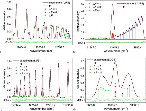
Hyperfine spectra of the Nb i lines measured with LIFS or LOGS together with the best fitted curve. The hyperfine components are marked by the difference ΔF of the total angular momenta of the lower and upper hyperfine levels. In the lower part of the each figure the residuals between experimental and best fitted curves are given, multiplied by the factor indicated at left side of the graphs. a) Example for a line with a rather well resolved hfs, fitted with coupled parameters for the Lorentzian width for each group of hfs components with same ΔF: transition from 13 145.71 cm^-1, J = 9/2 − → 25 199.81 cm^-1, J = 9/2 at λ_air = 829.365 nm or σ_vac = 12   054.10 cm^-1. b) Example for a partly resolved line, fitted with same parameter for the Lorentzian width for all hfs components and coupled intensity parameters for all hfs components with ΔF = 0: transition from 12 357.70 cm^-1, J = 9/2 −  → 24 203.05 cm^-1, J = 11/2 at λ_air = 843.981 nm or σ_vac = 11   845.35 cm^-1. c) Example for a line that looks like completely resolved, but most peaks include two or three hfs components: transition from 17 476.22 cm^-1, J = 11/2 −  → 30 191.25 cm^-1, J = 13/2 at λ_air = 786.255 nm or σ_vac = 12   715.03 cm^-1. d) Example for an unresolved line fitted with coupled profile parameters, B constants fixed to zero and fixed A constant of the lower level: transition from 19 568.72 cm^-1, J = 5/2 −  → 32 654.48 cm^-1, J = 5/2 at λ_air = 763.979 nm or σ_vac = 13   085.76 cm^-1.