| Issue |
A&A
Volume 556, August 2013
|
|
|---|---|---|
| Article Number | A8 | |
| Number of page(s) | 9 | |
| Section | Catalogs and data | |
| DOI | https://doi.org/10.1051/0004-6361/201321205 | |
| Published online | 17 July 2013 | |
Obliquity, precession rate, and nutation coefficients for a set of 100 asteroids⋆
1
Department of MathematicsUniversity of Rome Tor Vergata,
00133
Rome,
Italy
2
Observatoire de Paris, SYRTE/UMR-8630 CNRS,
75014
Paris,
France
e-mail:
This email address is being protected from spambots. You need JavaScript enabled to view it.
Received:
31
January
2013
Accepted:
18
April
2013
Abstract
Context. Thanks to various space missions and the progress of ground-based observational techniques, the knowledge of asteroids has considerably increased in the recent years.
Aims. Due to this increasing database that accompanies this evolution, we compute for a set of 100 asteroids their rotational parameters: the moments of inertia along the principal axes of the object, the obliquity of the axis of rotation with respect to the orbital plane, the precession rates, and the nutation coefficients.
Methods. We select 100 asteroids for which the parameters for the study are well-known from observations or space missions. For each asteroid, we determine the moments of inertia, assuming an ellipsoidal shape. We calculate their obliquity from their orbit (instead of the ecliptic) and the orientation of the spin-pole. Finally, we calculate the precession rates and the largest nutation components. The number of asteroids concerned leads to some statistical studies of the output.
Results. We provide a table of rotational parameters for our set of asteroids. The table includes the obliquity, their axes ratio, their dynamical ellipticity Hd, and the scaling factor K. We compute the precession rate ψ̇ and the leading nutation coefficients Δψ and Δε. We observe similar characteristics, as observed by previous authors that is, a significantly larger number of asteroids rotates in the prograde mode (≈ 60%) than in the retrograde one with a bimodal distribution. In particular, there is a deficiency of objects with a polar axis close to the orbit. The precession rates have a mean absolute value of 18″/y, and the leading nutation coefficients have an average absolute amplitude of 5.7″ for Δψ and 5.2″ for Δε. At last, we identify and characterize some cases with large precession rates, as seen in 25143 Itokawa, with has a precession rate of about − 475′′/y.
Key words: minor planets, asteroids: general / catalogs / methods: data analysis
Tables 1 and 2 are only available at the CDS via anonymous ftp to cdsarc.u-strasbg.fr (130.79.128.5) or via http://cdsarc.u-strasbg.fr/viz-bin/qcat?J/A+A/556/A8
© ESO, 2013
1. Introduction
The general knowledge of asteroids has been subject to tremendous progress in recent years thanks to very up-to-date ground-based observational techniques and to a significantly increasing number of space missions devoted to close approaches and exploration of these objects. In contrast to orbital parameters, which can generally be deduced precisely from a small set of positions and velocities that are recorded at a suitable interval of time, rotational characteristics of an asteroid necessitates high-frequency measurements. Most studies of these characteristics are based mainly on lightcurve profiles from which rotation rates and global shapes can be extracted. Lightcurve observations are generally not expensive in terms of equipment needed but require a lot of observing time to gather enough data for a precise solution of the spin vector.
In parallel to rotation rates and spin vector orientation, an estimation of the diameter of the asteroids can be obtained in both magnitude and distance determinations. When these results are collected for a large set of objects, statistical studies can be carried out on the distribution of rotation rates and diameters or on the distribution of the orientation of the spin vector with respect to the ecliptic (Pravec et al. 2002). Nevertheless, we note a lack of information concerning some parameters, when investigating the general data available for asteroids.
First, the estimation of the obliquity is generally not provided, and this is quite surprising, because obliquity is supposed to play a significant role in instances, such as resurfacing and space weathering. Indeed, obliquity directly determines the lengths and the contrasts of the seasons, which exist on the asteroids, and on the terrestrial planets, where these factors are fundamental. A large value of obliquity of an asteroid assumes that some parts of its surface are much more exposed to sunlight than others and that a climatic contrast exists, which is characterized by large differences in solar flux and solar wind exposure. In contrast, a value of obliquity close to zero implies that the solar influence should be the same for each part of the asteroid. These remarks are all available along the asteroidal year, which lasts a few terrestrial years for the main belt asteroids (MBAs).
Second, the precession rates and nutation coefficients of the asteroids are generally not
provided by a modern database. The rates and coefficients should be calculated when
considering the asteroids in a short-axis rotational state, which is generally confirmed by
the observations. Indeed, it was demonstrated theoretically that in the presence of
dissipation the equilibrium of a body in rotation is reached when it rotates around its
short-axis, which corresponds to the axis with a maximum moment of inertia (Kinoshita 1992), although long-axis mode rotations can
possibly be detected around tumbling objects (Burns &
Safronov 1973; Harris 1994). More precisely,
the energy-dissipation profile may be complex (Pravec et al.
2002), but a reasonable estimate on the timescale τ of damping of
the excited rotation to the lowest state of short-axis rotation ,assuming a low amplitude
libration, has been derived by (Burns & Safronov
1973):  (1)where μ is
the rigidity of the material composition of the asteroid, Q is the quality
factor, which expresses the ratio of the energy contained in the oscillation to the energy
lost per cycle, ρ is the bulk density of the body, and
(1)where μ is
the rigidity of the material composition of the asteroid, Q is the quality
factor, which expresses the ratio of the energy contained in the oscillation to the energy
lost per cycle, ρ is the bulk density of the body, and
 is a
dimensionless factor that is related to the shape of the body (with a value close to 0.01
for a quasi-spherical body to a value close to 0.1 for a highly elongated one).
R is the mean radius of the asteroid, and ω its angular
velocity of rotation. An alternative formula for τ was given by Harris (1994), who estimated the parameters in (1):
is a
dimensionless factor that is related to the shape of the body (with a value close to 0.01
for a quasi-spherical body to a value close to 0.1 for a highly elongated one).
R is the mean radius of the asteroid, and ω its angular
velocity of rotation. An alternative formula for τ was given by Harris (1994), who estimated the parameters in (1):
 (2)where
 is the
rotation period, D is the mean diameter, and C is a
constant close to 17 (with a factor ≈2.5 uncertainty). The parameter τ is
expressed here in billion of years, when P is in hours, and
D in km. Applying this law, it can be found that the damping timescale is
much shorter than the characteristic timescale of events, causing excitation of their
rotations as impacts or close encounters (Pravec et al.
2002).
is the
rotation period, D is the mean diameter, and C is a
constant close to 17 (with a factor ≈2.5 uncertainty). The parameter τ is
expressed here in billion of years, when P is in hours, and
D in km. Applying this law, it can be found that the damping timescale is
much shorter than the characteristic timescale of events, causing excitation of their
rotations as impacts or close encounters (Pravec et al.
2002).
As a consequence, the great majority of asteroids are rotating in a short-axis mode, which means that the axis of rotation should coincide with the axis of figure, which can be defined as the axis with the maximum moment of inertia. As for the Earth, the axis of figure of an asteroid (or its axis of rotation) is therefore supposed to exhibit a slow motion in space, known under the terminology, precession of equinoxes. The precession of equinoxes is because of the torque exerted principally by the Sun and comes from the fact that the asteroid is flattened at its equator. This motion is still verified when the asteroid has a well-pronounced triaxial shape, and when it is far from satisfying the conditions of axi-symmetry of the figure axis. In addition to the precession that is characterized by a conical loop with respect to the inertial space with the obliquity as an aperture angle and that is described in a timescale typically of several tens thousands of years, any asteroid should undergo small nutation oscillations that come from the gravitational torque exerted by the Sun on the flattened body.
Few studies of the combined precession-nutation motion of an asteroid have been carried out until now. For accurate modeling, we can mention Souchay et al. (2003b,a) for the asteroid 433 Eros, which follows the NEAR space mission and Rambaux et al. (2011) for 1 Ceres, the largest body of the asteroid belt. In this last and recent paper, the authors explain that owing to the small amplitudes of the nutation and the very long period of the precession motion, the measurements of the rotational variations of Ceres should be challenging to obtain by observational data as in the instance of the Dawn mission. They also estimated the timescale for Ceres orientation to relax to a generalized Cassini state, finding that the tidal dissipation within this asteroid has probably been too small to drive any significant damping of its obliquity since its formation. Nevertheless, it is worthy calculating the precession and nutation amplitudes for a large set of asteroids; a method is explained in the following section.
2. Precession and main nutation coefficients
Here, we assume that each given asteroid considered in the following can be assimilated to
a rigid body with a perfect ellipsoidal shape in which the moments of inertia
A,B,C satisfy
A < B < C,
with respect to the semi-axes a, b, c,
where
a < b < c.
Moreover, we only take into account the effects of the Sun on the rotation, which is
supposed to satisfy a short-axis mode, such that the rotation vector is very close to the
figure axis that is of length c. For each asteroid, the expression of the
disturbing potential exerted by the Sun in spherical harmonics limited at the first order is
(Kinoshita (1977)):
![Mathematical equation: \begin{eqnarray} U &=& {\kappa^2 M_{\rm S} \over r^3} \left( \left[{2C - A - B \over 2}\right] P_{2}^{0} (\sin \delta)\right. \notag\\ &&\left.\phantom{\left[{2C - A - B \over 2}\right]}+\, \left[{A - B\over 4} \right] P_{2}^{2}(\sin \delta) \cos 2 \alpha \right) , \end{eqnarray}](/articles/aa/full_html/2013/08/aa21205-13/aa21205-13-eq34.png) (3)where
κ2 is the gravitational constant,
MS is the mass of the Sun, and r the
heliocentric distance of the asteroid.
(3)where
κ2 is the gravitational constant,
MS is the mass of the Sun, and r the
heliocentric distance of the asteroid.  is the
associated Legendre polynomial and depends on the variable δ, which
represents the declination of the Sun with respect to the equator of the asteroid
(containing the semi-axes with lengths a and b). Here, the
variable α does not designate the right ascension of the Sun but its
longitude is counted from a prime meridian fixed to the asteroid. Therefore, the second term
of the right hand side of Eq. (3) denotes high frequency with a cycle corresponding to half
the rotational period of the asteroid due to the presence of the term
cos2α. For this reason it can be shown (Souchay et al. 2003a) that this part of the potential does not participate to the
precession and gives birth to very small nutation coefficients. Thus, we do not take it into
account here.
is the
associated Legendre polynomial and depends on the variable δ, which
represents the declination of the Sun with respect to the equator of the asteroid
(containing the semi-axes with lengths a and b). Here, the
variable α does not designate the right ascension of the Sun but its
longitude is counted from a prime meridian fixed to the asteroid. Therefore, the second term
of the right hand side of Eq. (3) denotes high frequency with a cycle corresponding to half
the rotational period of the asteroid due to the presence of the term
cos2α. For this reason it can be shown (Souchay et al. 2003a) that this part of the potential does not participate to the
precession and gives birth to very small nutation coefficients. Thus, we do not take it into
account here.
In order to compute the precession rate and the leading nutation coefficient, we follow exactly the same procedure as Souchay et al. (2003b) when they precisely studied the rotation of the asteroid 433 Eros. For that purpose, they followed a complete analytical theory of the rotation of a rigid body in Hamiltonian formalism, which was developed by Kinoshita (1977), and applied to the Earth with a very high level of accuracy (Souchay et al. 1999).
Through the intermediary of Jacobi polynomials, the Legendre polynomial
 can be
split into three components, involving the longitude of the Sun
λS, its latitude βS that is
defined with respect to an arbitrary reference plane and an arbitrary starting point, and
I which is the inclination of the asteroid equator that is defined with
respect to this basic plane.
can be
split into three components, involving the longitude of the Sun
λS, its latitude βS that is
defined with respect to an arbitrary reference plane and an arbitrary starting point, and
I which is the inclination of the asteroid equator that is defined with
respect to this basic plane. ![Mathematical equation: \begin{eqnarray} P_{2}^{0} (\sin \delta) &=& {1 \over 2} \left(3 \cos^2 J -1\right) \left[{1 \over 2} \left(3 \cos^2 I -1\right) P_{2}^{0}(\sin \beta_{\rm S})\right.\notag\\ &&- \,{1 \over 2} \sin 2 I P_{2}^{1} \left(\sin \beta_{\rm S}\right) \sin \left(\lambda_{\rm S} -h\right)\notag\\ &&\left. -\, {1 \over 4} \sin^2 I P_{2}^{2} \left( \sin \beta_{\rm S}\right) \cos 2 \left(\lambda_{\rm S} -h\right) \right] , \end{eqnarray}](/articles/aa/full_html/2013/08/aa21205-13/aa21205-13-eq46.png) (4)where
J represents the angle between the directions of the angular momentum
vector and of the figure axis. This angle is supposed to be very small in general, as it is
for the Earth for which it does not exceed 1″. It has never been detected for the other
terrestrial planets, which supports the hypothesis that this smallness is also satisfied for
them. Therefore, we can postulate that also for the asteroids investigated here. The
variable h is also a very small quantity, varying very slowly compared to
λ, which represents the displacement of the starting point along the
reference plane (Souchay et al. 2003b,a). It can be neglected if compared to λ
at first order.
(4)where
J represents the angle between the directions of the angular momentum
vector and of the figure axis. This angle is supposed to be very small in general, as it is
for the Earth for which it does not exceed 1″. It has never been detected for the other
terrestrial planets, which supports the hypothesis that this smallness is also satisfied for
them. Therefore, we can postulate that also for the asteroids investigated here. The
variable h is also a very small quantity, varying very slowly compared to
λ, which represents the displacement of the starting point along the
reference plane (Souchay et al. 2003b,a). It can be neglected if compared to λ
at first order.
We have seen above that the basic plane from which obliquity, precession, and nutation are
computed is arbitrary. A judicious choice is to take for this plane the orbital plane of the
asteroid around the Sun, so that the latitude βS is equal to
zero. Thus,  In
that case, this leads to the final simplified formula for U:
In
that case, this leads to the final simplified formula for U:
![Mathematical equation: \begin{equation} U = k \left[{a \over r}\right]^3 \times \left[-{1 \over 4} \left(3 \cos^2 I -1\right) -{3 \over 4} \sin^2 I \cos (2 \lambda_{\rm S} -h) \right] \end{equation}](/articles/aa/full_html/2013/08/aa21205-13/aa21205-13-eq53.png) (8)with
(8)with
![Mathematical equation: \begin{equation} k = {\kappa^2 M_{\rm S} \over a^3} \left[{2C - A - B \over 2}\right] \cdot \end{equation}](/articles/aa/full_html/2013/08/aa21205-13/aa21205-13-eq54.png) (9)With the specific
choice of the basic plane above, I represents the obliquity:
I = ε.
(9)With the specific
choice of the basic plane above, I represents the obliquity:
I = ε.
2.1. Precession rate
The precession rate ψ̇
for any asteroid is calculated in a very straightforward manner by integrating the
constant part of the potential in (8) (Kinoshita
1977; Souchay et al. 2003b). It is given
by the following expression at the fourth order of the eccentricity:
![Mathematical equation: \begin{equation} \dot \psi = {K \over 2} \times \left[ 1 + {3 \over 2} e^2 + {15 \over 4} e^4 \right] \cos \varepsilon , \end{equation}](/articles/aa/full_html/2013/08/aa21205-13/aa21205-13-eq56.png) (10)where the expression
in brackets, which depends on the sole eccentricity, corresponds to the constant part of
the quantity (a/r)3. The
scaling factor K is given at first order by:
(10)where the expression
in brackets, which depends on the sole eccentricity, corresponds to the constant part of
the quantity (a/r)3. The
scaling factor K is given at first order by:
 (11)where
Hd = (2C − A − B/2C)
represents the dynamical ellipticity of the asteroid, which is characterized by its
flattening. The parameter n stands for the mean motion of the asteroid
and ω for its angular rotational velocity.
(11)where
Hd = (2C − A − B/2C)
represents the dynamical ellipticity of the asteroid, which is characterized by its
flattening. The parameter n stands for the mean motion of the asteroid
and ω for its angular rotational velocity.
2.2. Nutation coefficients
The nutation characterizes the small oscillations undergone by the pole of figure (or
rotation) in space. It is obtained by keeping the solar potential periodic (sinusoidal)
components. It is characterized by the oscillations of the obliquity Δε
and of the longitude of the node Δψ between the equator of figure and the
orbital plane of the asteroid. As expressed in a simplified manner by Souchay et al. (2003b,a), which starts from the formula in Kinoshita
(1977), the nutations in longitude Δψ and in obliquity
Δε can be approximated at first order by
![Mathematical equation: \begin{eqnarray} \Delta \psi &=& {K \cos \varepsilon \over 2} \times \int \left[ \left[ {a\over r}^3 \right] - \left[ {a\over r}^3 \right] \cos\left(2 \lambda_{\rm S} - 2h\right) {\rm d}t \right]_{\rm per.} , \\ \Delta \varepsilon &=& {K \over 2} \times \int \left[ \left[ {a\over r}^3 \right] \sin \left(2 \lambda_{\rm S} - 2h\right) {\rm d}t \right]_{\rm per.} . \end{eqnarray}](/articles/aa/full_html/2013/08/aa21205-13/aa21205-13-eq61.png) Here,
the index per. means that we only keep the periodic
(sinusoidal) part of the expression.
Here,
the index per. means that we only keep the periodic
(sinusoidal) part of the expression.
After integration, Δψ and Δε are given in the form of
Fourier series with the same formalism as Souchay et al.
(2003b) for Eros 433. By keeping only the leading components, we have
![Mathematical equation: \begin{eqnarray} \Delta \psi\!\! &\approx& \! {K \cos \varepsilon \over 2} \left[\! -\left(1\! - \!{5 \over 2} e^2\right) {\sin 2 \lambda \over 2 \dot \lambda}\! + \!{ 3 e \sin M \over \dot M}\!+\! {e \over 2} {\sin \lambda \over \dot \lambda} \!+ \!\cdots \right] \!,\quad\quad\\ \Delta \varepsilon\! &\approx& \! {K \sin \varepsilon \over 2} \left[ \left(1 - {5 \over 2} e^2\right) {\cos 2 \lambda \over 2 \dot \lambda} - {e \over 2} {\cos \lambda \over \dot \lambda} + \cdots \right] , \end{eqnarray}](/articles/aa/full_html/2013/08/aa21205-13/aa21205-13-eq63.png) where
M is the mean anomaly of the asteroid, whereas λ
stands for its longitude, which is counted from the equinoctial point that is defined from
the ascending node of the Sun relative orbital plane with respect to the asteroid
equatorial plane. Because of the very slow motion of the asteroid equinoxes, the linear
rates,
where
M is the mean anomaly of the asteroid, whereas λ
stands for its longitude, which is counted from the equinoctial point that is defined from
the ascending node of the Sun relative orbital plane with respect to the asteroid
equatorial plane. Because of the very slow motion of the asteroid equinoxes, the linear
rates,  and Ṁ, can be considered as identical at first approximation. Therefore,
the sinusoidal expressions with arguments of the form sinM and
sinλ in Eq. (14) can be considered as having the same frequency with a
phase shift that varyies very slowly with time.
and Ṁ, can be considered as identical at first approximation. Therefore,
the sinusoidal expressions with arguments of the form sinM and
sinλ in Eq. (14) can be considered as having the same frequency with a
phase shift that varyies very slowly with time.
We note that the period of the largest nutation oscillation in Δψ is either the orbital period of the asteroid (component with sinM) or half this period (component with sin2λ), according to the value of the eccentricity. In the case of Δε this indetermination does not exist for the term, where the argument M does not exist. Therefore, the leading oscillation has always a semi-orbital period with argument 2λ.
3. The available database
To carry out our computations of obliquity, precession, and nutation, according to Eqs. (14) and (15), our study is based on the following four electronic databases:
-
(1)
Planetary Data System Asteroid/Dust Archive1,
-
(2)
Database of Asteroid Models from Inversion Techniques2,
-
(3)
IAU Minor Planet Center3,
-
(4)
Wolfram Curated Data (AstronomicalData)4.
The shape models of various asteroids and complementary information on the spin can be found in the Database of Asteroid Models from Inversion Techniques (DAMIT). The database not only contains well-curated data obtained from lightcurves of asteroids but also provides a compilation of additional asteroid data and relevant references. See the webpage of Durech et al. (2010) for more information.
The orbital elements are taken from the IAU Minor Planet Center (MPC), from the MPC Orbit (MPCORB) database. It contains the orbital elements of minor planets that have been published in the Minor Planet Circulars, the Minor Planet Orbit Supplement, and the Minor Planet Electronic Circulars.
Both data on rotational and orbital aspects of about 50 000 asteroids can also be found in the AstronomicalData product of the Wolfram Curated Data (WCD; see webpage for further references). The data can be directly accessed through Wolfram Mathematica or through the Wolfram Alpha webpage. The database was used to cross-reference the orbital and rotational data if sufficient data are available. In the following, we refer (1)−(4) to the content of the databases taken from PDS, DAMIT, MPC and WCD, respectively.
3.1. General information
For the asteroids that were visited during space missions, data are taken from the web and from (1)−(4) (see also short discussion in Sect. 3.2). For all remaining asteroids the missing physical properties are taken from (1) and (2), and the orbital elements are taken from (3). All data are obtained in the following way: i) only objects, which are present in all four databases were taken into account. ii) the mass (if available) and radius of an individual object are obtained from (4), where the radius is cross-checked with the diameter published in (2). iii) the ratios of the semi axes a/b and b/c are taken from (1), and the numbers are cross-referenced with the ratios obtained from (2) by fitting an ellipsoid through the published shape models using a standard least squares method (see also Sect. 4). This also provides, in addition to a/b and b/c, the axis c in physical units. Note that depending on the numbers of shape models published for one object in (2), we may obtain more than one solution for a/b, b/c, and c from the latter database. The rotation period of an individual object is taken from (2) and is cross-referenced with the rotation period of the same object published in (4). The spin-pole position of an asteroid in ecliptic coordinates (λ,β) is taken from (2) (given at epoch J2000); the values are cross-referenced with the spin-pole positions also published in (1). In the latter, the positions are given in terms of (λ,β) but at epoch B1950.
We note that up to four spin-pole positions may be found in (1) for one individual asteroid (the number depends on the method of determination of the spin-pole positions). In that specific case the positions come in two pairs of solutions (one value of one pair shifted by about 180° from the second one). The orbital period is taken from (4), while the orbital elements are obtained from (3). There are cases, where all necessary data about the orbit, the spin vector and the geometry can be found in (1), but the asteroid is not listed in (2). The asteroids were added to our target list too. In total we were able to keep seven asteroids with data obtained from space missions, 34 asteroids with data from (1) and (2) and 59 asteroids with enough information from (1) but not from (2). Thus, we finally gathered 100 asteroids from which we have enough data to deduce the obliquity and precession periods.
We provide our target list (see Table 1) in which one data point entry consists of four lines. Each line starts with the IAU designation number of the asteroid:
1:id., name,
2:id., m[1] , [4], R[4] [km], a/b[1], b/c[1], no., c[2] [km], a/b[2], b/c[2],
3:id., ![Mathematical equation: \hbox{$T_{rot}^{[2],[4]}[h]$}](/articles/aa/full_html/2013/08/aa21205-13/aa21205-13-eq87.png) ,
λ[2], β[2],
ε[2] , [3], no.,
λ[1],
β[1],ε[1] , [3],
,
λ[2], β[2],
ε[2] , [3], no.,
λ[1],
β[1],ε[1] , [3],
4:id.,![Mathematical equation: \hbox{$T_{rev}^{[4]}[y]$}](/articles/aa/full_html/2013/08/aa21205-13/aa21205-13-eq94.png) ,
T0[3],
a[3] [AU],
e[3], i[3],
ω[3], Ω[3],
M[3], n[3][°/d].
,
T0[3],
a[3] [AU],
e[3], i[3],
ω[3], Ω[3],
M[3], n[3][°/d].
In line1 id. stands for the designation number, and name is the official IAU name of the object, as published in (3). In line2: m, taken from (1) or (4), is the mass of the object given in the mass unit of Ceres; the equatorial radius R is given in [km]; the first two ratios, a/b and b/c, are the ratios of the semi axes published in (1); no. defines the number of shape models that exist for one asteroid in (2) from which a,b,c and the respective ratios are calculated (see below).
In line3, Trot is the rotation period (in hours) of the asteroid as published in (2). The first three parameters (λ,β,ε) denote the ecliptic longitude λ and latitude β as they are published in (2); the resulting obliquity ε has been calculated on the basis of the orbital parameters (line 4). The integer no. gives the number of spin-vector solutions, which are published for one object in (1) (the number of triplets of the form (λ,β,ε) that could be calculated using the different (λ, β) that are published in (1) on the basis of the orbital parameters given in line4).
The first entry in line4 is the orbital period in [y] published in (4), T0 defines the epoch for which the elements are given; a is the semi-major axis in [AU]; e is the eccentricity, i is the inclination, ω is the argument of perihelium; Ω is the longitude of the ascending node; M is the mean anomaly at T0, and n is the mean motion in [°] and [°/d]. We note that all values are taken as they are published in (1)−(4) with the exception of the second set of shape parameters a/b,b/c, and c in line2, which were calculated from shape models published in (2) and the obliquities of the asteroids ε in line3. The obliquities are obtained by combining the spin-vector solutions, which are published in (1) or (2) with the orbital parameters (published for the object in (3) and (4)) according to a method fully described in Sect. 5.
3.2. Complementary information from space missions
For some asteroids that have been visited during space missions, additional information is available: NASA’s space probe Galileo (launched 1989) was the first to make a flyby near an asteroid (951 Gaspra) and discovered the first asteroid moon (Dactyl) around the asteroid 243 Ida. The NEAR Shoemaker mission (launched 1996) was designed to study the near-Earth asteroid 433 Eros in great detail over a period of a year and was the first probe to touch down on an asteroid surface (2001 Feb. 12). It also flew by the asteroid 253 Mathilde. The Deep Space 1 spacecraft (launched 1998), maintained by NASA, carried out a flyby of asteroid 9969 Braille and included an encounter with the comet, Borelly. For cost reasons, the asteroid 1999 KK1 was not visited by the spacecraft at the end of the mission.
The primary aim of the space mission named Stardust (launched 1999) was to collect dust samples from the coma of the comet Wild 2; but however it also flew by and studied the asteroid 5535 Annefrank. In 2000, the Cassini space probe passed the asteroid 2685 Masursky on its way to the planet Saturn. Another space mission called CONTOUR (launched 2002) investigated the nuclei of the two comets, Encke and Schwassmann-Wachmann-3, but did not visit an asteroid. The JAXA mission named Hayabusa, formerly known as MUSES-C (launched 2003), visited the asteroid 25143 Itokawa with the aim of returning the first sample of the surface of the asteroid back to Earth. The mission also included a lander (MINERVA), which unfortunately failed to reach the surface. An important contribution is from the European robotic spacecraft mission Rosetta (launched 2004), to study the comet 67P/Churyumov-Gerasimenko in 2014. However, the space probe already completed its flybys of the asteroid 2867 Steins (2008), the asteroid P/2012 A2, and 21 Lutetia (2010). The space probe, Deep Impact (launched in 2005), visited the comet 9P/Tempel and will reach the asteroid (163249) 2002GT within the year 2020. The asteroid 4 Vesta was already visited by NASA’s DAWN spacecraft during 2011, 2012 with the aim to reach the dwarf planet Ceres in 2015.
Future missions with possible flybys of asteroids or minor planets include: the NASA mission New Horizons, which already had its closest approach with the asteroid 132524 APL in the year 2006; the Chinese space probe Chang’e 2, which will visit the asteroid 4179 Toutatis; the JAXA mission Hayabusa 2 (targeting the asteroid 162173 1999 JU3 with a lander called MASCOT, which is going to be developed at the DLR in collaboration with the French space agency CNES; Don Quijote, which is a proposed space probe by the European Space Agency to investigate the effects of crashes into an asteroid (2003 SM84 or 99942 Apophis); the US space mission OSIRIS-REx, which aims to return a sample from the asteroid 1999 RQ36; the ESA mission AIDA with possible target 65803 Didymos; and the MarcoPolo-R mission, which in the framework of the Cosmic Vision program is supposed to return a sample from the binary asteroid system (175706) 1996 FG3. In total, we found 14 asteroids, which were visited during space missions in the last 30 years. We could collect enough data for only seven of them for the purpose of the present calculations.
4. Computation of the moments of inertia
For any given asteroid, the principal moments of inertia
A < B < C
are linked to the second degree spherical harmonics by
 (16)where
M and R are the mass and radius of the asteroids and
where the coefficients J2 and c22
can be obtained from experiments in space. However, only a few asteroids have been visited
by space probes so far, and we are able to determine the gravity field for only a few of
them. As a consequence, J2 and c22
are unknown for the majority of the asteroids, and we cannot use them to calculate
A,B and C directly. As a first approximation, we assume
that the asteroid is of uniform density and can be approximated by an ellipsoidal shape. In
that case, the principal moments of inertia are given by Bills & Nimmo (2011):
(16)where
M and R are the mass and radius of the asteroids and
where the coefficients J2 and c22
can be obtained from experiments in space. However, only a few asteroids have been visited
by space probes so far, and we are able to determine the gravity field for only a few of
them. As a consequence, J2 and c22
are unknown for the majority of the asteroids, and we cannot use them to calculate
A,B and C directly. As a first approximation, we assume
that the asteroid is of uniform density and can be approximated by an ellipsoidal shape. In
that case, the principal moments of inertia are given by Bills & Nimmo (2011):
 (17)Here a,b
and c are the semi axes of the fitting ellipsoid, and M is
the mass of the asteroid, which is also not known with enough accuracy for the large
majority of asteroids. Nevertheless we can have access to the ratios,
a/b and
b/c, which can be estimated directly
from observations (from the shape of the asteroid itself obtained from lightcurve inversion
techniques Kaasalainen & Torppa 2001; Kaasalainen et al. 2001).
(17)Here a,b
and c are the semi axes of the fitting ellipsoid, and M is
the mass of the asteroid, which is also not known with enough accuracy for the large
majority of asteroids. Nevertheless we can have access to the ratios,
a/b and
b/c, which can be estimated directly
from observations (from the shape of the asteroid itself obtained from lightcurve inversion
techniques Kaasalainen & Torppa 2001; Kaasalainen et al. 2001).
In (2), different shape models are given for an individual asteroid in the form of
polyhedrons with triangular surface facets in terms of vertex coordinates
(xi,yi,zi) ∈ R3
with i = 1,...,N ∈N and
order numbers  for each facet
with j = 1,...,M ∈N. For
our purpose, only the vertex coordinates are used: the data points fit an ellipsoid with
free parameters a,b and c through them by making use of a
standard least squares method. We thus aim to minimize the quantity,
for each facet
with j = 1,...,M ∈N. For
our purpose, only the vertex coordinates are used: the data points fit an ellipsoid with
free parameters a,b and c through them by making use of a
standard least squares method. We thus aim to minimize the quantity,
 (18)with respect to the
unknown parameters (a,b,c), where
i = 1,...,N. The
typical number of points N used in the fitting process are on the order of
102 to 103. Moreover, the typical absolute errors (absolute
difference of di from zero) ranges from a
fraction of 1 percent to 10 percent of the mean radius. We note that the final values
(a,b,c) in a few cases are switched to follow the usual convention
a ≥ b ≥ c. We indicate this by a ∗ and
+ in Table 2.
(18)with respect to the
unknown parameters (a,b,c), where
i = 1,...,N. The
typical number of points N used in the fitting process are on the order of
102 to 103. Moreover, the typical absolute errors (absolute
difference of di from zero) ranges from a
fraction of 1 percent to 10 percent of the mean radius. We note that the final values
(a,b,c) in a few cases are switched to follow the usual convention
a ≥ b ≥ c. We indicate this by a ∗ and
+ in Table 2.
In our ongoing calculations, we only need the dynamical ellipticity
Hd, which is given by
![Mathematical equation: \begin{equation} H_{\rm d}=\frac{2C-A-B}{2C}=\frac{1}{2}-\left[\left(\left(\frac{a}{b}\right)^2+1\right) \left(\frac{b}{c}\right)^2\right]^{-1} , \end{equation}](/articles/aa/full_html/2013/08/aa21205-13/aa21205-13-eq145.png) (19)where the right hand-side
comes from the contribution of (17) combined with the middle of (19). As we can see,
Hd has become independent of the mass M, and
only the ratios a/b and
b/c take part to its calculation. We
are thus able to take into account all the asteroids for which only the relative ratios of
the semi-axes are known, even if the masses are usually not. To test the validity of our
approach we also use the algorithm described in Mirtich
(1996) to directly calculate the principal moments of inertia matrix from the shape
models that are published in (2). Let us denote
ex,ey,ez
the eigenvectors, and
λx,λy,λz
the coresponding eigenvalues of the moments of inertia matrix. From the formulae,
2/5ma2 = λy + λz − λx
and
2/5mb2 = λz + λx − λy,
2/5mc2 = λx + λy − λz,
we are able to obtain the ratios a/b
and b/c, without fitting an ellipsoid
to the data set.
(19)where the right hand-side
comes from the contribution of (17) combined with the middle of (19). As we can see,
Hd has become independent of the mass M, and
only the ratios a/b and
b/c take part to its calculation. We
are thus able to take into account all the asteroids for which only the relative ratios of
the semi-axes are known, even if the masses are usually not. To test the validity of our
approach we also use the algorithm described in Mirtich
(1996) to directly calculate the principal moments of inertia matrix from the shape
models that are published in (2). Let us denote
ex,ey,ez
the eigenvectors, and
λx,λy,λz
the coresponding eigenvalues of the moments of inertia matrix. From the formulae,
2/5ma2 = λy + λz − λx
and
2/5mb2 = λz + λx − λy,
2/5mc2 = λx + λy − λz,
we are able to obtain the ratios a/b
and b/c, without fitting an ellipsoid
to the data set.
5. Determination of obliquities
The obliquity of each asteroid is a fundamental parameter for our calculations. We
calculate the value of the obliquity ε from the knowledge of the spin and
orbit poles of the asteroid. First, the direction of the spin pole, f, is
defined in terms of its ecliptic longitude λ and latitude
β by  (20)Second, the unit vector
with a direction parallel to the orbit pole, o, which is normal to the
asteroid’s orbit, is given by
(20)Second, the unit vector
with a direction parallel to the orbit pole, o, which is normal to the
asteroid’s orbit, is given by  (21)The obliquity
ε can be obtained by inverting the two following formulae:
(21)The obliquity
ε can be obtained by inverting the two following formulae:
 (22)where w is
the unit vector along the direction of the descending node of the asteroid’s orbit with
respect to the true equator. In (1), (λ,β) are given with respect to J2000;
in (2), they are given with respect to B1950. To transform from B1950 to J2000, we simply
add 0.7° to the ecliptic
longitude λ, which is accurate enough, since the accuracy of the spin pole
positions is typically about a few degrees.
(22)where w is
the unit vector along the direction of the descending node of the asteroid’s orbit with
respect to the true equator. In (1), (λ,β) are given with respect to J2000;
in (2), they are given with respect to B1950. To transform from B1950 to J2000, we simply
add 0.7° to the ecliptic
longitude λ, which is accurate enough, since the accuracy of the spin pole
positions is typically about a few degrees.
If the spin pole is given in the equatorial coordinate system in terms of the declination
δ and right ascension α, these coordinates can be easily
transformed to the ecliptic system by (Bills & Nimmo
(2011))  (23)If we define the rotation
matrix R1 = R1(ϕ)
about the angle ϕ as
(23)If we define the rotation
matrix R1 = R1(ϕ)
about the angle ϕ as
 (24)the
(q1,q2,q3)
can be calculated from
(24)the
(q1,q2,q3)
can be calculated from  (25)where
εE stands for the obliquity of the Earth. That is
εE = 23°26′21.448′′ (J2000).
(25)where
εE stands for the obliquity of the Earth. That is
εE = 23°26′21.448′′ (J2000).
6. Presentation of basic tables
In this section we collect the main results of our study, consisting of 100 asteroids for which we were able to calculate the obliquity, precession rate, and nutation coefficients (Table 2).
The quality of our data is mainly limited by the accuracy of the observations and measurements at the present day. Out of hundreds of thousands of known asteroids, we only collected data from 100 asteroids for which the dynamical ellipticity and the obliquity, which are crucial in the calculation of the precession rates and nutation coefficients, could be determined with enough accuracy.
Moreover, the published values for a/b and b/c are determined with known errors and oversimplified assumptions, such as the assumption that the shapes of asteroids are ellipsoids. As a result, our results strongly depend on the method that the authors used to determine them and as a consequence, different values exist for the same object.
 |
Fig. 1 Pairs of obliquities, (ε1,ε2), found for the same asteroid but taken from different data sources (top), pairs of shape parameters, ((a/b)1,(a/b)2) and (b/c)1,(b/c)2, for the same asteroid but from different data sources (bottom). The plot markers indicate the different source of the data, see text. |
To get an idea of the widespread values of obliquities, we plot two estimations of them against each other in the upper plot of Fig. 1. In other words, we have pairs of obliquities (ε1,ε2), of the same asteroid taken from two different databases. The values range from 17° to 172°. With the exception of a few outliers, we can remark that the values, which we have calculated in both cases from the published values of the spin- and orbit-axes directions with Eq. (22) are in good agreement.
The situation is different when we compare the ratios a/b and b/c for the asteroids that are common in the two different databases, that were obtained from the two different shape models, or that were determined through the two different methods, as described in Sect. 4. Indeed, we find more than one solution for the ratios of 34 asteroids among our set of 100 objects (see Fig. 1): similar to the pairs of obliquites (ε1,ε2), we found different pairs of ratios (a/b)1,(a/b)2 and (b/c)1,(b/c)2 for the same asteroid that were taken from two different data sources. This is due to the different shape models and different determination of these ratios. The deviation of the filled disks (squares) from the median indicates the difference of the ratios a/b and b/c originating from different shape models; filled diamonds (triangles) reveal the difference of the ratios a/b (b/c) due to the two determination methods. We clearly see that the uncertainty in the shape models is about the order of magnitude of the error that we introduced when fitting just an ellipsoid. It is thus safe to use the first method, as described in Sect. 4 to obtain the values a/b and b/c for the ongoing calculations. The uncertainty in these ratios directly affects the uncertainty in the dynamical ellipticity Hd. We will address the issue one more time in the following section (Fig. 4).
7. Results and statistics
In the following discussion we split our dataset into three different sets:
-
db1 contains the data of the asteroids for which it was possible to find information for the shape and for the spin- and orbit-axes from which we calculated the obliquity in both (1) and (2).
-
db2 contains the data for which this same information (enabling the deduction of ε, a/b and b/c) can only be found in (2) but not in (1).
-
db3 concerns the asteroids for which (generally accurate) data are taken from space missions.
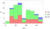 |
Fig. 2 Distribution of obliquities for 100 asteroids for different subsets db1, db2, db3 and all of them. |
The results on the obliquites of the asteroids of our solar system are shown in Fig. 2: the obliquites range from
 with a median value of
about 75°. On the basis of our
data, we find significantly less asteroids within the interval -20° (or 160°)
to 20°. We remark that no
asteroid was found between -8° (172°) to 8°. Moreover, we also find
a relative deficiency of asteroids with large obliquity which means that their polar axis is
close to the orbit (and generally to the ecliptic). Only eight objects (2, Pallas, 7 Iris, 8
Flora, 16 Psyche, 22 Kalliope, 28 Bellona, 433 Eros, and 704 Interamnia) are found in the
range
80° < ε < 100°.
This conforms the remark made by Michalowski (1993)
and also agrees with Magnusson (1986, 1990) who analyzes the spin vectors of 20 to 30 asteroids
respectively. When quoting the apparent lack of poles with axes close to the ecliptic, this
last author attributed this deficiency to an observational selection effect: an asteroid
with a pole at a low ecliptic latitude is naturally less suitable to present a significant
amplitude of the lightcurve variation. He concluded that these asteroids needed more
lightcurve observations than for an asteroid with a polar axis close to the ecliptic. Drummond et al. (1988, 1991) confirmed the bimodality of the observed pole distribution using results for
26 asteroids. If they used the same explanation as Magnusson
(1986, 1990) for this distribution, they did
not exclude the possibility that the bimodality may be real and may reflect a primordial
distribution of spin rates. Another confirmation of the non-uniform distribution of spin
axes comes from Pravec et al. (2002), who use a
larger sample of asteroid-pole estimates than the authors above. Their dataset comes mainly
from two databases, the NASA Planetary Data System and the Uppsala’s website, which is
completed by other studies. Their sample with a total of 83 asteroids showed once more that
the distribution of obliquities is bimodal and not flat. They carried out a
Kolmogorov-Smirnov test, showing that the distribution is not uniform at a 85% confidence
level.
with a median value of
about 75°. On the basis of our
data, we find significantly less asteroids within the interval -20° (or 160°)
to 20°. We remark that no
asteroid was found between -8° (172°) to 8°. Moreover, we also find
a relative deficiency of asteroids with large obliquity which means that their polar axis is
close to the orbit (and generally to the ecliptic). Only eight objects (2, Pallas, 7 Iris, 8
Flora, 16 Psyche, 22 Kalliope, 28 Bellona, 433 Eros, and 704 Interamnia) are found in the
range
80° < ε < 100°.
This conforms the remark made by Michalowski (1993)
and also agrees with Magnusson (1986, 1990) who analyzes the spin vectors of 20 to 30 asteroids
respectively. When quoting the apparent lack of poles with axes close to the ecliptic, this
last author attributed this deficiency to an observational selection effect: an asteroid
with a pole at a low ecliptic latitude is naturally less suitable to present a significant
amplitude of the lightcurve variation. He concluded that these asteroids needed more
lightcurve observations than for an asteroid with a polar axis close to the ecliptic. Drummond et al. (1988, 1991) confirmed the bimodality of the observed pole distribution using results for
26 asteroids. If they used the same explanation as Magnusson
(1986, 1990) for this distribution, they did
not exclude the possibility that the bimodality may be real and may reflect a primordial
distribution of spin rates. Another confirmation of the non-uniform distribution of spin
axes comes from Pravec et al. (2002), who use a
larger sample of asteroid-pole estimates than the authors above. Their dataset comes mainly
from two databases, the NASA Planetary Data System and the Uppsala’s website, which is
completed by other studies. Their sample with a total of 83 asteroids showed once more that
the distribution of obliquities is bimodal and not flat. They carried out a
Kolmogorov-Smirnov test, showing that the distribution is not uniform at a 85% confidence
level.
Another factor of study concerns the relative amount of prograde/retrograde rotations. If we neglect db3, which is not statistically representative (for it contains only 7 asteroids), for each of the samples considered in our study, the number of asteroids having ε < 90° (prograde case) is significantly larger than the opposite (retrograde case), as can be seen in Fig. 2. For the whole sample, we have 57 prograde objects against 43 retrograde ones. These values that translate into percentages (using the complete set of 100 asteroids) are in very good agreement with those found by Pravec et al. (2002), who found 48 prograde rotations versus 32 retrograde ones. These values correspond respectively to 60% and 40% of their sample.
Moreover, it is worthy to mention an important point: all the authors quoted above in this section consider the obliquity of the spin axis with respect to the ecliptic, whereas we calculate the true obliquity, which is characterized by the angle between the spin axis and the orbital one in this study. The difference between the values deduced from the two methods could reach (in the optimal case) the value of the inclination of the orbit of the asteroid with respect to the ecliptic, which corresponds to a substantial amount (more, and sometimes much more than 10°) in some cases. Therefore, the statistics of these authors should be a little affected by their approximate method of calculation. Nevertheless, it is true that the corresponding error should be compensated by the uncertainty concerning the spin axis orientation itself, which is generally determined with error bars of a few degrees.
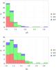 |
Fig. 3 Distribution of a/b (top) and b/c (bottom) for 100 asteroids for the different subsets (db1, db2, db3) and for all of them. |
In Fig. 3, we report the distribution of the shape parameters a/b and b/c. We can remark in particular that values of the ratios a/b and b/c are significantly more probable to be found close to 1 than values far from unity. The median values for these ratios are both close to 1.2. However, one should notice that the distribution is biased because the shape parameters cannot be derived easily and usually exhibit large error bars (see bottom of Fig. 1).
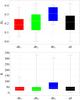 |
Fig. 4 Distribution of Hd (top) and K (bottom) for 100 asteroids for the different subsets (db1, db2, db3) and for all of them. The filled rectangle marks the 75% quantile. Lines bound the upper and lower range, the center line marks the median value of the respective data set. |
The distributions of the dynamical ellipticity Hd and of the
scaling factor K, which plays a direct and fundamental role in the
amplitude of the precession rate and nutation coefficients, are shown in Fig. 4. The median value of Hd in
db1 lies close to 0.184 and increases to 0.226 for db2
and 0.310 for db3. In the global data set, we find a median value of about
0.215. The values seem to be randomly distributed with large variations (between 0 and
0.423, as seen in the error bars), with a confidence interval between 0.128 and 0.286. Some
statistics on the scaling factor K are shown in Fig. 4 (bottom), ranging from 0 to 330″/y
(881″/y for the outlier 25143 Itokawa) with a median
value of about 33″/y. We notice that the dynamical
ellipticity for the Earth, which is rather poorly flattened with respect to the objects
studied here, is  , and
the scaling factor KEarth for the Sun part of the potential (our
sole interest here) is
KEarth = 34.38″/y.
Therefore, the values of Hd are typically larger by one or two
orders than for our planet, as we can see from Table 1 or Table 2, but the values of
K are of the same order.
, and
the scaling factor KEarth for the Sun part of the potential (our
sole interest here) is
KEarth = 34.38″/y.
Therefore, the values of Hd are typically larger by one or two
orders than for our planet, as we can see from Table 1 or Table 2, but the values of
K are of the same order.
In Fig. 5 we collect the results on the precession
rate (top figure) and the leading nutation coefficients. We remark that we adopt the same
conventions for the sign of the precession rate as for the Earth. This means that a positive
sign characterizes a retrograde motion of the equinox. Moreover, this sign depends only on
the value of the obliquity with respect to 90°, as can be checked in Eq. (8). As
a consequence of the distribution of the obliquities discussed above, most of the asteroids
are found to have ψ̇ positive for our four data sets. As we can deduce from Table 2, the mean absolute value of
this rate is 18.07″/y, which can be compared with the
solar part of the precession of the Earth (15″/y) and
the combined lunisolar part (≈50″/y). In most of the
cases here, the absolute value of the precession rate has smaller amplitudes than this last
value, with the exception of 25143 Itokawa ( ), 624 Hektor
(
), 624 Hektor
( ), 60 Echo
(
), 60 Echo
( ), 277 Elvira
(
), 277 Elvira
( ), and 71 Niobe
(
), and 71 Niobe
( ).
).
The absolute values of the leading nutation coefficients in longitude
Δψ1 for the semi-annual oscillation (half the orbital period)
and Δψ2 for the annual one are given simultaneously for all the
objects of our sample. For Δψ1, the distributions deduced from
Table 2 are shown in Fig. 5 (upper middle). They range
between 0″ and 41″ (for 23145 Itokawa) with a mean value of about
 . The distribution is quite
similar for Δψ2 (see lower middle of Fig. 5) with a minimum value at 0″, a maximum value around 93″ (still for 23145
Itokawa), and a mean value of about , which is close to the case of
Δψ1. The mean absolute value of Δψ (taken as
the sup of Δψ1 and Δψ2) is
. The distribution is quite
similar for Δψ2 (see lower middle of Fig. 5) with a minimum value at 0″, a maximum value around 93″ (still for 23145
Itokawa), and a mean value of about , which is close to the case of
Δψ1. The mean absolute value of Δψ (taken as
the sup of Δψ1 and Δψ2) is
 .
.
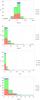 |
Fig. 5 Distribution of ψ̇ (top), Δψ1 (upper middle), Δψ2 (lower middle) and Δε (bottom) for 100 asteroids for the different subsets (db1, db2, db3) and for all of them. |
Our final study concerns the nutation coefficient Δε in Fig. 5 (bottom): we find  , with a median value of
 and a mean value of
 . To compare with the Earth, the
leading nutation due to the sole solar gravitational effect is semi-annual with absolute
amplitudes – roughly 1″ for Δψ and
. To compare with the Earth, the
leading nutation due to the sole solar gravitational effect is semi-annual with absolute
amplitudes – roughly 1″ for Δψ and  for Δε.
Therefore, the solar nutation amplitudes of the asteroids are generally significantly larger
than for our planet.
for Δε.
Therefore, the solar nutation amplitudes of the asteroids are generally significantly larger
than for our planet.
8. Conclusion
In the present study, we calculated a complete set of the obliquities, precession rates and nutation coefficients for a sample of 100 (out of about 550 000 known) asteroids for the first time. For our calculations we extracted the relevant data from four main databases for which the shape parameters a/b and b/c are known (or can be calculated from shape models) to be able to determine the dynamical ellipticity Hd and the scaling parameter K. We selected only the asteroids for which the spin-pole position is well determined, to calculate the obliquity ε that is needed to deduce the precession rate ψ̇ and the leading nutation coefficients, Δψ and Δε. Our calculations were based on the theory of the rotational motion of a rigid body developed by Kinoshita (1977) and have already been applied for the asteroid Eros 433 by Souchay et al. (2003b,a). We present all our results in form of a database of 100 asteroids in Table 2. The relevant data to construct this table is presented in Table 1.
Thanks to our relatively large sample of 100 asteroids, we were able to analyze the asteroid data and to derive some statistical properties of the rotational characteristics. Concerning the distribution of obliquities, main features are revealed, which agree with previous authors (Drummond et al. (1988, 1991); Magnusson (1986, 1990); Michalowski (1993); Pravec et al. (2002)). However, the results in these studies are affected, because they aproximated the orbital plane by the ecliptic for the calculation of the obliquity, while we used the true orbital plane that enabled us to calculate the more accurate value of the obliquity.
In our study, the obliquities of the asteroids are spread over the interval
9° ≤ ε ≤ 170° with the most
representative value of about 75°, which shows that
objects in the prograde rotation regime are significantly more numerous than those in the
retrograde one. The mean precession rate ψ̇
of the asteroids was found to be 2.87″/y, and its mean
absolute value is
 , which is comparable to the
amplitude of the solar component precession of the Earth
(15″/y). The nutation coefficients are typically on
the order of a few arcseconds; the mean absolute value for the leading term are
for Δψ and
, which is comparable to the
amplitude of the solar component precession of the Earth
(15″/y). The nutation coefficients are typically on
the order of a few arcseconds; the mean absolute value for the leading term are
for Δψ and
 for Δε. All
these values can reach significantly larger values for some specific objects, such as for as
60 Echo, 71 Niobe, 624 Hektor, and 277 Elvira. The largest values are obtained for 25143
Itokawa with
for Δε. All
these values can reach significantly larger values for some specific objects, such as for as
60 Echo, 71 Niobe, 624 Hektor, and 277 Elvira. The largest values are obtained for 25143
Itokawa with
 and
and
 . Corresponding to a precession
cone described in only 2725 years, this supposes a very fast precession motion, which may be
detectable from lightcurves within two or three decades.
. Corresponding to a precession
cone described in only 2725 years, this supposes a very fast precession motion, which may be
detectable from lightcurves within two or three decades.
In conclusion, this paper constitutes an interesting work to better understand the evolution of the rotational motion of the asteroids. In particular, it presents a statistical analysis of the precession rates and nutations of the asteroids for the first time. It extends statistical studies to a larger set of objects, to computations of the obliquity variations, and to the precession-nutation effects.
Wolfram Mathematica or http://www.wolframalpha.com/
References
- Bills, B. G., & Nimmo, F. 2011, Icarus, 213, 496 [NASA ADS] [CrossRef] [Google Scholar]
- Burns, J. A., & Safronov, V. S. 1973, MNRAS, 165, 403 [NASA ADS] [CrossRef] [Google Scholar]
- Drummond, J. D., Weidenschilling, S. J., Chapman, C. R., & Davis, D. R. 1988, Icarus, 76, 19 [NASA ADS] [CrossRef] [Google Scholar]
- Drummond, J. D., Weidenschilling, S. J., Chapman, C. R., & Davis, D. R. 1991, Icarus, 89, 44 [NASA ADS] [CrossRef] [Google Scholar]
- Durech, J., Sidorin, V., & Kaasalainen, M. 2010, A&A, 513, A46 [NASA ADS] [CrossRef] [EDP Sciences] [Google Scholar]
- Harris, A. W. 1994, Icarus, 107, 209 [NASA ADS] [CrossRef] [Google Scholar]
- Kaasalainen, M., & Torppa, J. 2001, Icarus, 153, 24 [NASA ADS] [CrossRef] [Google Scholar]
- Kaasalainen, M., Torppa, J., & Muinonen, K. 2001, Icarus, 153, 37 [NASA ADS] [CrossRef] [Google Scholar]
- Kinoshita, H. 1977, Celest. Mech., 15, 277 [Google Scholar]
- Kinoshita, H. 1992, Celest. Mech. Dyn. Astron., 53, 365 [NASA ADS] [CrossRef] [Google Scholar]
- Magnusson, P. 1986, Icarus, 68, 1 [NASA ADS] [CrossRef] [Google Scholar]
- Magnusson, P. 1990, Icarus, 85, 229 [NASA ADS] [CrossRef] [Google Scholar]
- Michalowski, T. 1993, Icarus, 106, 563 [NASA ADS] [CrossRef] [Google Scholar]
- Mirtich, B. 1996, J. Graph. Tools, 31, 1 [Google Scholar]
- Pravec, P., Harris, A. W., & Michalowski, T. 2002, Asteroids III, 113 [Google Scholar]
- Rambaux, N., Castillo-Rogez, J., Dehant, V., & Kuchynka, P. 2011, A&A, 535, A43 [NASA ADS] [CrossRef] [EDP Sciences] [Google Scholar]
- Souchay, J., Loysel, B., Kinoshita, H., & Folgueira, M. 1999, A&AS, 135, 111 [NASA ADS] [CrossRef] [EDP Sciences] [Google Scholar]
- Souchay, J., Folgueira, M., & Bouquillon, S. 2003a, EMP, 93, 107 [Google Scholar]
- Souchay, J., Kinoshita, H., Nakai, H., & Roux, S. 2003b, Icarus, 166, 285 [NASA ADS] [CrossRef] [Google Scholar]
All Figures
|
Fig. 1 Pairs of obliquities, (ε1,ε2), found for the same asteroid but taken from different data sources (top), pairs of shape parameters, ((a/b)1,(a/b)2) and (b/c)1,(b/c)2, for the same asteroid but from different data sources (bottom). The plot markers indicate the different source of the data, see text. |
| In the text | |
|
Fig. 2 Distribution of obliquities for 100 asteroids for different subsets db1, db2, db3 and all of them. |
| In the text | |
|
Fig. 3 Distribution of a/b (top) and b/c (bottom) for 100 asteroids for the different subsets (db1, db2, db3) and for all of them. |
| In the text | |
|
Fig. 4 Distribution of Hd (top) and K (bottom) for 100 asteroids for the different subsets (db1, db2, db3) and for all of them. The filled rectangle marks the 75% quantile. Lines bound the upper and lower range, the center line marks the median value of the respective data set. |
| In the text | |
|
Fig. 5 Distribution of ψ̇ (top), Δψ1 (upper middle), Δψ2 (lower middle) and Δε (bottom) for 100 asteroids for the different subsets (db1, db2, db3) and for all of them. |
| In the text | |
Current usage metrics show cumulative count of Article Views (full-text article views including HTML views, PDF and ePub downloads, according to the available data) and Abstracts Views on Vision4Press platform.
Data correspond to usage on the plateform after 2015. The current usage metrics is available 48-96 hours after online publication and is updated daily on week days.
Initial download of the metrics may take a while.